The blog will consist of the steps to create a primary neural network, starting from understanding matrix multiplication to building your training loop. Apart from building the neural net, I will discuss various customisation techniques as well. Let us begin this journey.


Step:1 — MatMul
Today, we will learn the first step to building the Neural network, and it is the primary matrix multiplication. There are many ways to do so, and we will see each one and will compare them to get the best results.
We require matrix multiplication in the linear layer of the Neural Networks. To do matrix multiplication, we need a dataset. Fastai is kind to provide various datasets, and we will use the MNIST dataset to do operations.
So, let’s grab the dataset.
- Firstly, I am importing the libraries that I will use throughout the series.
- After that, I am downloading the MNIST dataset with the extension
.gzprovided. - Since the file downloaded was in pickle format; therefore, I am using the function
pickle.loadto access the dataset. - Dataset downloaded is the numpy arrays, and we want PyTorch tensors to perform operations in regards to the Neural Networks. Therefore, I am using
mapfunction to map the numpy array to torch tensors. - Thus, our dataset is ready.


weights = torch.randn(784,10)
bias = torch.zeros(10)m1 = x_valid[:5]
m2 = weightsm1.shape,m2.shape
  = (torch.Size([5, 784]), torch.Size([784, 10]))
Type — 1: Simple Python Programme
We can do matrix multiplication using the simple python programs. But python programs take a lot of time to implement and let us see how.
%timeit -n 10 t1=matmul(m1, m2)


- 847 ms is a lot of time when we have only five rows in the validation dataset.
Type — 2: Element wise Operations
Pytorch provided us with an effortless way to do matrix multiplications, and it is known as element-wise operations. Let us understand it.
- We have eliminated the last loop.
- In the element-wise operation, the multiplying units are considered as the Rank-1 tensors.
m2[:, 1].shape
  = torch.Size([784])m1[1, :].shape
  = torch.Size([784])
- The above code runs in C. Let us see the time taken by it to execute.
%timeit -n 10 t1=matmul(m1, m2)


Type — 3: Broadcasting
Broadcasting is another way of matrix multiplication.
As per the Scipy docs, the term broadcasting describes how numpy treats arrays with different shapes during arithmetic operations. Subject to certain constraints, the smaller array is “broadcast” across the larger array so that they have compatible shapes. Broadcasting provides a means of vectorising array operations so that looping occurs in C instead of Python. It does this without making needless copies of data and usually leads to efficient algorithm implementations. Broadcasting happens a C speed and with CUDA speed on GPU.
m1[2].unsqueeze(1).shape
  = torch.Size([784, 1])
- In broadcasting, the entire column of the input having dimensions as [1 * 784] is squeezed to [784 * 1] and then multiplied with the weights.
- Finally, the sum is taken across the column as
sum(dim=0)and is stored in thec.
%timeit -n 10 _=matmul(m1, m2)


Type — 4: Einstein summation
Einstein summation (
einsum) is a compact representation for combining products and sums in a general way.
From the numpy docs:
“The subscripts string is a comma-separated list of subscript labels, where each label refers to a dimension of the corresponding operand.”
“The subscripts string is a comma-separated list of subscript labels, where each label refers to a dimension of the corresponding operand.”
- It is a more compact representation.
- The number of inputs represents the rank of input
ikdesignates rank-2 tensor,kjdesignates rank-2 tensor. - The dimension of a matrix is represented as
i*k,k*jandi*j. - Whenever you see the repeated dimension, do dot product over that dimension.
%timeit -n 10 _=matmul(m1, m2)


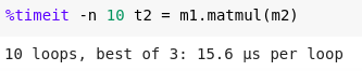
Type — 5: PyTorch Operation
We can use PyTorch’s function or operator directly for matrix multiplication.
%timeit -n 10 t2 = m1.matmul(m2)

%timeit -n 10 t2 = m1@m2

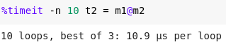
Thus, we can easily compare the timings of various codes. This is the reason also that we do not prefer to write the code in the Python language due to its slow performance. Therefore, most of the python libraries are implemented in the C.
Step:2&3 — Relu/init & Forward pass
After we have defined the matrix multiplication strategy, its time to defined the ReLU function and the forward pass for the Neural Network. I would request the readers to go through the Part — 1 of the series to get the background of the data used below.
The Neural Network is defined as below:
output = MSE(Linear(ReLU(Linear(X))))
Basic Architecture
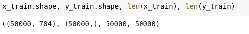
n,m = x_train.shape
c = y_train.max()+1
n,m,c


Let us explain the weights for the matrix multiplication.
I will create a 2-layer neural network.
- The first linear layer will do the matrix multiplication of the input with w1.
- The output of the first linear layer will be the input for the second linear operation, where the input will be multiplied with the w2.
- Instead of getting ten predictions for a single input, I will obtain the single output and will use MSE to calculate the loss.
- Let us declare the weights and biases.
w1 = torch.randn(m,nh)
b1 = torch.zeros(nh)w2 = torch.randn(nh,1)
b2 = torch.zeros(1)
- When we declare the weights and biases using the PyTorch
randn, then the weights and biases obtained are normalized, i.e. they have a mean of 0 and a standard deviation of 1. - We need to normalise the weights and biases so that they do not lead to substantial values after the linear operation with the input to the Neural Network. Because large outputs become difficult for the computers to handle. Therefore, we prefer to normalise the inputs.


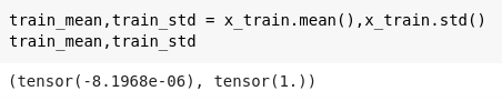
- For the same reason, we want out input matrix to have a mean of 0 and a standard deviation of 1, which is not at present. Lets us see.
train_mean,train_std = x_train.mean(),x_train.std()
train_mean,train_std


- Let us define a function to normalise the input matrix.
def normalize(x, m, s): return (x-m)/sx_train = normalize(x_train, train_mean, train_std)
x_valid = normalize(x_valid, train_mean, train_std)
- Now, we are normalising the training dataset and the validation dataset on the same mean and standard deviation so that our training and validation dataset has the same feature definitions and scale. Now, let’s recheck the mean and standard deviation.

- Now, we have normalised weights, biases, and input matrix.
Let us define the linear layer for the Neural Network and perform the operation.
def lin(x, w, b): return x@w + bt = lin(x_valid, w1, b1)
t.mean(),t.std()

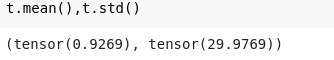
Now, the mean and standard deviation obtained after the linear operation is again non-normalized. Now, the problem is still pure. If it remains like this, more linear operations will lead to significant and substantial values, which will be challenging to handle. Thus, we want our activations after the linear operation to be normalized as well.
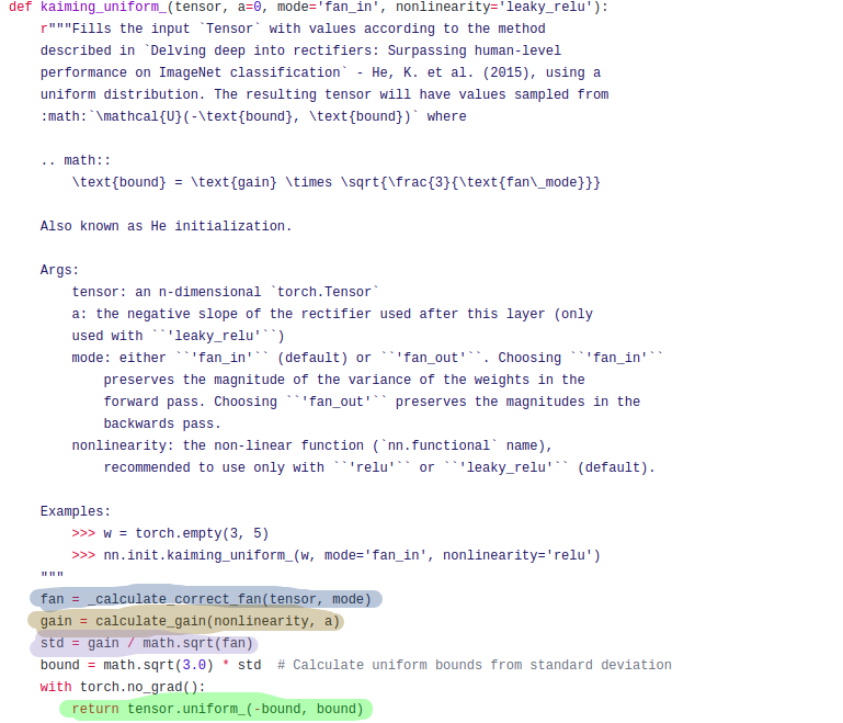
Simplified Kaiming Initialization or He Initialization
To handle the non-normalized behaviour of linear neural network operation, we define weights to be Kaiming initialized. Though Kaiming Normalization or He initialisation is defined to handle ReLu/Leaky ReLu operation, we still can use it for linear operations.

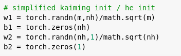
We divide our weights by math.sqrt(x) where x is the number of rows.
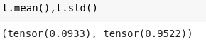
After the above trivia, we get the normalized mean and SD.
def lin(x, w, b): return x@w + bt = lin(x_valid, w1, b1)
t.mean(),t.std()

Let us define the ReLU layer for the Neural Network and perform the operation. Now, why we are defining the ReLU as a non-linear activation function, I hope you are aware of the Universal Approximation Theorem.
def relu(x): return x.clamp_min(0.)
t = relu(lin(x_valid, w1, b1))t.mean(),t.std()


t = relu(lin(x_valid, w1, b1))
t = relu(lin(t, w2, b2))t.mean(),t.std()


Did you notice something weird?
Notice above that our standard deviation gets halved of the one obtained after the linear operation, and if it gets halved after one layer, imagine after eight layers it will get to 1/²⁸, which is very very small. And if our neural network has got 10000 layers 😵, forget about it.
From PyTorch docs:
a: the negative slope of the rectifier used after this layer (0 for ReLU by default)
a: the negative slope of the rectifier used after this layer (0 for ReLU by default)

This was introduced in the paper that described the Imagenet-winning approach from Kaiming He and others: Delving Deep into Rectifiers, which was also the first paper that claimed “super-human performance” on Imagenet (and, most importantly, it introduced ResNets!)
Thus, following the same strategy, we will multiply our weights with
math.sqrt(2/m) .w1 = torch.randn(m,nh)*math.sqrt(2/m)t = relu(lin(x_valid, w1, b1)) t.mean(),t.std()


Though we have better results, still the mean is not so good. As per the fastai docs, We could handle the mean by the below tweak.
def relu(x): return x.clamp_min(0.) - 0.5w1 = torch.randn(m,nh)*math.sqrt(2./m )
t1 = relu(lin(x_valid, w1, b1))
t1.mean(),t1.std()


Let us combine the above all code and strategies and create the forward pass of our Neural Network. PyTorch has a defined method for Kaiming Normalization i.e
kaiming_normal_ .def model(xb): l1 = lin(xb, w1, b1) l2 = relu(l1) l3 = lin(l2, w2, b2) return l3%timeit -n 10 _=model(x_valid)


The last to be defined for the forward pass is the Loss function: MSE.
As per our previous knowledge, we generally use
CrossEntroyLoss as the loss function for single-label classification functions. I will address the same later. For now, I am using MSE to understand the operation.def mse(output, targ): return (output.squeeze(-1) - targ).pow(2).mean()
Let us perform the above operations for the training dataset.
preds = model(x_train)
preds.shape, preds


To perform the MSE, we need the floats.
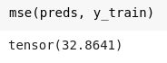
y_train,y_valid = y_train.float(),y_valid.float()mse(preds, y_train)

After all of the above operation, one question is still not answered substantially and it is
Why do we need Kaiming Initialization?
Let us understand it again.
Initialise two tensors as below.
import torchx = torch.randn(512)
a = torch.randn(512,512)
For Neural Networks, the primary step is the matrix multiplication and if we have a deep neural network with approx 100 layers, then let us see what will the standard deviation and mean of the activations obtained.
for i in range(100):
    x = x @ ax.mean(), x.std()


We can easily see that mean, and a standard deviation is no longer a number. And it is justified as well. The computer is not able to store that large numbers; it cannot account for such large numbers. It has restricted the practitioners to train such deep neural networks for the same reason.
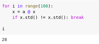
The problem you’ll get with that is activation explosion: very soon, your activations will go to nan. We can even ask the loop to break when that first happens:
for i in range(100):
    x = x @ a
    if x.std() != x.std(): breaki

Thus, such problems lead to the invention of Kaiming Initialization. It surely took decades to come up with the idea finally.
So, that’s how we define the ReLu and backward pass for the neural network.
Step:4 — Backward Pass
Till now, we have understood the idea behind the matrix multiplication, the ReLu function, and the forward pass of the Neural Network. Now, we will discuss the backward pass.
Before going into the backward pass, Lets us understand one question.
What is backpropagation?
This is the fancy term for the deep learning practitioners, especially when you are discussing with someone. But, in simpler terms, backpropagation is just calculating gradients through the chain rule. We find a gradient concerning the weights/parameters. It is this simple. Backpropagation is just the reverse of the gradient of the forward pass.
So let us find the gradients step by step.
— The gradient of the MSE layer
def mse(output, targ): return (output.squeeze(-1) — targ).pow(2).mean()def mse_grad(inp, targ):
# grad of loss with respect to output of previous layer
inp.g = 2. * (inp.squeeze() - targ).unsqueeze(-1) / inp.shape[0]
- We calculate the gradient of the input layer, which is the output of the previous layer. The gradient of MSE is defined as
2(predicted — target)/mean. - Since calculating gradients form the chain rule, we need to store the gradients of each layer, which gets multiplied to the previous layer. For this reason, we are saving the gradients in the
inp.ginput layer because it is the output layer in the prior layer.
— The gradient of the ReLU


Now, for any value greater than 0, we have to replace it with 0, and for values smaller than 0, we have to keep them 0.
def relu(x): return x.clamp_min(0.)def relu_grad(inp, out):
# grad of relu with respect to input activations
inp.g = (inp>0).float() * out.g
- We are multiplying the gradients of the previous layer which is the output layer for the ReLU i.e.
out.g. - This defines the chain rule.
— The gradient of the Linear layer
I found the gradient of the linear layer more challenging to understand than the other layers. But I will try my best to simplify it.
def lin(x, w, b): return x@w + bdef lin_grad(inp, out, w, b):
# grad of matmul with respect to weights
inp.g = out.g @ w.t()
w.g = (inp.unsqueeze(-1) * out.g.unsqueeze(1)).sum(0)
b.g = out.g.sum(0)
- inp.g — First, we calculate the gradient of the linear layer concerning the parameters.
- w.g — Gradient of weights
- b.g — Gradient of bias concerning the weights.
Now, let us combine both forward pass and backward pass.
def forward_and_backward(inp, targ):# forward pass:
    l1 = inp @ w1 + b1
    l2 = relu(l1)
    out = l2 @ w2 + b2
    # we don't actually need the loss in backward!
    loss = mse(out, targ)# backward pass:
    mse_grad(out, targ)
    lin_grad(l2, out, w2, b2)
    relu_grad(l1, l2)
    lin_grad(inp, l1, w1, b1)
forward_and_backward(x_train, y_train)
What if we compare the gradients we calculated with the gradients calculated by the PyTorch.
Before comparison, we need to store our gradients.
w1g = w1.g.clone()
w2g = w2.g.clone()
b1g = b1.g.clone()
b2g = b2.g.clone()
We cheat a little bit and use PyTorch autograd to check our results.
xt2 = x_train.clone().requires_grad_(True)
w12 = w1.clone().requires_grad_(True)
w22 = w2.clone().requires_grad_(True)
b12 = b1.clone().requires_grad_(True)
b22 = b2.clone().requires_grad_(True)
Let us define the forward function to calculate the gradients using the PyTorch.
def forward(inp, targ):
    # forward pass:
    l1 = inp @ w12 + b12
    l2 = relu(l1)
    out = l2 @ w22 + b22
    # we don't actually need the loss in backward!
    return mse(out, targ)loss = forward(xt2, y_train)
loss.backward()
Let us compare the w2 gradients.
w22.grad.T, w2g.T


Now, there are so many ways in which we can refactor the above-written code, but that is not the concern. We need to understand the semantics behind the backward pass of the Neural Networks. This is how we define backwards pass in our model.
Step:4(b) — kaiming Initialization for Convolutional network
In the previous part, we looked for the need of Kaiming Initialization for stabilising the effects of non-linear activation action. Now, the major for now is to see how kaiming initalization is used for Convolutional Networks. I will also tell you how it is implemented in PyTorch. So let us start the learning journey.
Background
From the last chapters, we have the below values.
x_train.shape, y_train.shape, x_valid.shape, y_valid.shape


Let us look into the shape of the dataset.
x_train[:100].shape, x_valid[:100].shape


From our knowledge of convolutional networks, Let us create a simple convolutional neural network using PyTorch.
import torch.nn as nnnh=32
l1 = nn.Conv2d(1, nh, 5)
- The number of input layers to the CNN is 1.
- The number of output filters or layers are 32.
5represents the kernel size.
When we are talking of Kaiming initialization, the first thing that comes to the mind is to calculate the mean and standard deviation of weights of the convolutional neural network.
def stats(x): return x.mean(),x.std()
l1 has defined weights in it. Let’s understand them before calculating the stats.
l1.weight.shape


As per the weights:
32represents the number of output layers/filters.1represents the number of input layers5, 5represents the kernel size.
We need to focus on the output of the convolutional neural network.
x = x_valid[:100]
# you may train the neural network using the training dataset but for now, I am taking vaidation daaset. There is no specific reason behind it.x.shape


100— number of images1— input layer.28, 28— dimensions of the input image.
t = l1(x)
t.shape


100— number of images32— number of output layers24, 24— kernel size
stats(t)

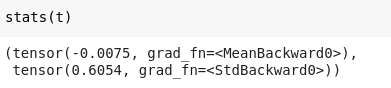
But, we want the standard deviation of 1 instead of 0.6, though we have a mean of 0. So, let us apply kaiming initialization to the weights.
init.kaiming_normal_(l1.weight, a=1.)
stats(l1(x))


Now, it is better. Mean is almost 0 and SD is around 1.
But, kaiming initialization was introduced to handle the non-linear activation function. Let us define it.
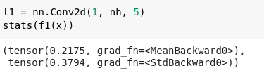
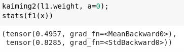
import torch.nn.functional as Fdef f1(x,a=0): return F.leaky_relu(l1(x),a)init.kaiming_normal_(l1.weight, a=0)
stats(f1(x))


— Mean is not around 0, but SD is almost equal to 1.
Without kaiming initialization, let us find the stats.
l1 = nn.Conv2d(1, nh, 5)
stats(f1(x))

- Now, you can easily compare the stats with and without the kaiming.
- With kaiming, results are much better.
Compare
Now, let us compare our results with the PyTorch. Before that, we need to see the PyTorch code.
torch.nn.modules.conv._ConvNd.reset_parameters


kaiming_uniform

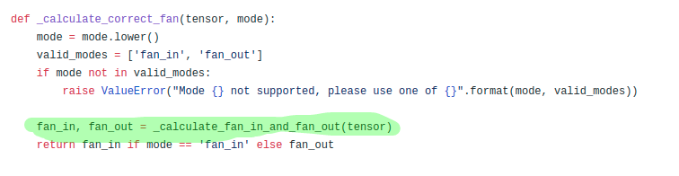
calculate_correct_fan

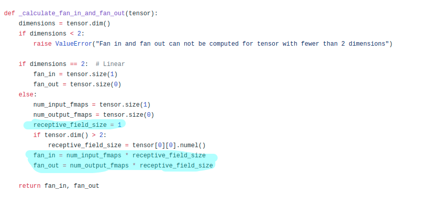
calculate_fan_in_fan_out

Let us understand the above methods.
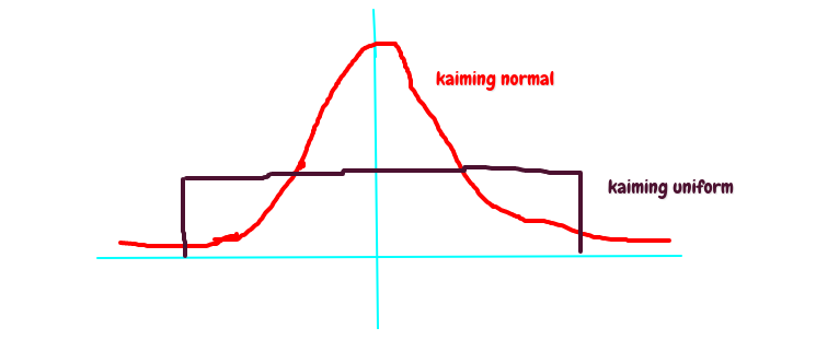
- PyTorch uses kaiming_uniform instead of kaiming_normal. The kaiming_uniform is different from the later in terms of the value boundaries.

- There is a variable
receptive_field_sizein calculate_fan_in_fan_out(). It is calculated as below.
l1.weight.shape
  = torch.Size([32, 1, 5, 5])l1.weight[0,0].shape
  = torch.Size([5, 5])rec_fs = l1.weight[0,0].numel()
rec_fs


fan_in(number of input parameters)andfan_out(number of output filters)are calculated as below.
nf,ni,*_ = l1.weight.shape
nf,ni


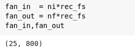
fan_in  = ni*rec_fs
fan_out = nf*rec_fsfan_in,fan_out

- There is one more parameter
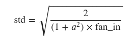
gainin kaiming_uniform(). It is the amount of leakiness in the non-linear activation function. It is defined as below.
def gain(a): return math.sqrt(2.0 / (1 + a**2))
- For ReLU, the value of a is 0. Therefore, the value of gain for ReLU is math.sqrt(2.0). Look into the below link.
From all the above knowledge, we can create our kaiming_uniform as below.
def kaiming2(x,a, use_fan_out=False):
    nf,ni,*_ = x.shape
    rec_fs = x[0,0].shape.numel()
    fan = nf*rec_fs if use_fan_out else ni*rec_fs
    std = gain(a) / math.sqrt(fan)
    bound = math.sqrt(3.) * std
    x.data.uniform_(-bound,bound)
Let us calculate the stats.
kaiming2(l1.weight, a=0);
stats(f1(x))

The results are still better.
So, this is how kaiming concept is used in the Convolutional Neural Networks.
Step:5 — Training Loop
Now, we have reached to the point where we need to know about the CrossEntropy loss because mainly CrossEntropy loss is used in single or multi-classification problems. Since we are using MNIST dataset, then we need to create a neural network which will predict for ten numbers, i.e. from 0 to 9. Earlier, we used the MSE loss and predicted the single outcome, which we generally do not do.
So before learning the loss function deeply, let us create a neural network using PyTorch nn.module.
from torch import nn
class Model(nn.Module):
    def __init__(self, n_in, nh, n_out):
        super().__init__()
        self.layers = [nn.Linear(n_in,nh), nn.ReLU(),      nn.Linear(nh,n_out)]

    def __call__(self, x):
        for l in self.layers: x = l(x)
            return x
We have below-defined variables.
n,m = x_train.shape
c = y_train.max()+1
nh = 50
Let us defined the weights again.
w1 = torch.randn(m,nh)/math.sqrt(m)
b1 = torch.zeros(nh)
w2 = torch.randn(nh,10)/math.sqrt(nh)
b2 = torch.zeros(10)
You may observe the differences in the weight initialization. This time, we want ten predictions, one for each number in the output. That is why I initialized w2 to be (nh, 10).
model = Model(m, nh, 10)
pred = model(x_train)pred.shape


— Cross entropy loss
Again, before indulging into the Cross-Entropy loss, we need to take softmax of our predictions or activations. We do softmax in the case; we want single-label classification. In practice, we will need the log of the softmax when we calculate the loss because it helps further in calculating the cross-entropy loss.
Softmax is defined as:


or more concisely:


def log_softmax(x): return (x.exp()/(x.exp().sum(-1,keepdim=True))).log()
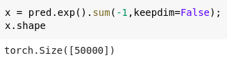
x.exp().sum(-1,keepdim=True)will sum the exponentials of the activations along the row.- If
keepdimisTrue, the output tensor is of the same size asinputexcept in the dimensiondimwhere it is of size 1. Otherwise,dimis squeezed, resulting in the output tensor having one fewer dimension thaninput.


Since we have defined the
log_softmax , let us take the log_softmax of our predictions.sm_pred = log_softmax(pred)


The cross-entropy loss is defined as below:
def CrossEntropy(yHat, y):
    if y == 1:
      return -log(yHat)
    else:
      return -log(1 - yHat)
In binary classification, where the number of classes M equals 2, cross-entropy can be calculated as:
−(𝑦log(𝑝)+(1−𝑦)log(1−𝑝))
If M>2 (i.e. multiclass classification), we calculate a separate loss for each class label per observation and sum the result.


Our problem is multiclass classification, so our cross-entropy loss function would be later one. The cross-entropy loss function for multiclass classification can also be done using numpy-style integer array indexing. Let us implement using it.
def nll(input, target): return -input[range(target.shape[0]), target].mean()
loss = nll(sm_pred, y_train)
Note that the formula


gives a simplification when we compute the log softmax, which was previously defined as
(x.exp()/(x.exp().sum(-1,keepdim=True))).log() .def log_softmax(x): return x - x.exp().sum(-1,keepdim=True).log()
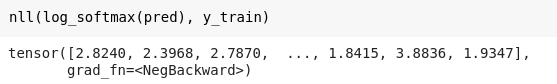
loss = nll(log_softmax(pred), y_train)
Then, there is a way to compute the log of the sum of exponentials in a more stable way, called the LogSumExp trick. The idea is to use the following formula:


- Take out the maximum value from the predictions.
- Subtract the maximum value from the exponential of the predictions.
- At last, add the maximum value to the log of the operation, as suggested in the above image.
- It helps in the computation and makes it faster without affecting the output in either case.
Let us define our LogSumExp.
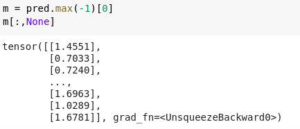
m = pred.max(-1)[0]
m[:,None]

def logsumexp(x):
    m = x.max(-1)[0]
    return m + (x-m[:,None]).exp().sum(-1).log()
So we can use it for our
log_softmax function.def log_softmax(x): return x - x.logsumexp(-1,keepdim=True)

Let us see the above implementation in PyTorch.
import torch.nn.functional as F
F.nll_loss(F.log_softmax(pred, -1), y_train)
In PyTorch,F.log_softmaxandF.nll_lossare combined in one optimized function,F.cross_entropy.
— Basic training loop
The training loop repeats over the following steps:
- get the output of the model on a batch of inputs
- compare the output to the labels we have and compute a loss
- calculate the gradients of the loss with respect to every parameter of the model
- update the parameters/weights with those gradients to make them a little bit better.
- repeat the above steps at loop known as
epochs.
Let us combine all the above concepts and create our loop.
bs = 64
lr = 0.5   # learning rate
epochs = 1 # how many epochs to train for
So, this is how we define the training loop in the neural loop. Now, in PyTorch, it has some syntax differences which you can understand now. I will add more steps to this series with time. Till then, feel free to explore it.


No comments:
Post a Comment