Feature Selection and Dimensionality Reduction Using Covariance Matrix Plot

This article will discuss how the covariance matrix plot can be used for feature selection and dimensionality reduction.
Why are feature selection and dimensionality reduction important?
A machine learning algorithm (such as classification, clustering or regression) uses a training dataset to determine weight factors that can be applied to unseen data for predictive purposes. Before implementing a machine learning algorithm, it is necessary to select only relevant features in the training dataset. The process of transforming a dataset in order to select only relevant features necessary for training is called dimensionality reduction. Feature selection and dimensionality reduction are important because of three main reasons:
- Prevents Overfitting: A high-dimensional dataset having too many features can sometimes lead to overfitting (model captures both real and random effects).
- Simplicity: An over-complex model having too many features can be hard to interpret especially when features are correlated with each other.
- Computational Efficiency: A model trained on a lower-dimensional dataset is computationally efficient (execution of algorithm requires less computational time).
Dimensionality reduction, therefore, plays a crucial role in data preprocessing.
We will illustrate the process of feature selection and dimensionality reduction with the covariance matrix plot using the cruise ship dataset cruise_ship_info.csv. Suppose we want to build a regression model to predict cruise ship crew size based on the following features: [‘age’, ‘tonnage’, ‘passengers’, ‘length’, ‘cabins’, ‘passenger_density’]. Our model can be expressed as:


where X is the feature matrix, and w the weights to be learned during training. The question we would like to address is the following:
Out of the 6 features [‘age’, ‘tonnage’, ‘passengers’, ‘length’, ‘cabins’, ‘passenger_density’], which of these are the most important?
We will determine what features will be needed for training the model.
The dataset and jupyter notebook file for this article can be downloaded from this repository: https://github.com/bot13956/ML_Model_for_Predicting_Ships_Crew_Size.
1. Import Necessary Libraries
import numpy as np
import pandas as pd
import matplotlib.pyplot as plt
import seaborn as sns
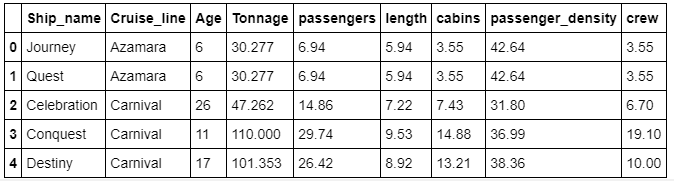
2. Read dataset and display columns
df=pd.read_csv("cruise_ship_info.csv")
df.head()

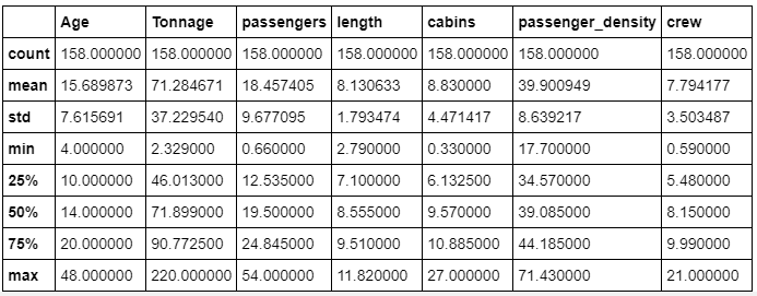
3. Calculate basic statistics of the data
df.describe()

4. Generate Pairplot
cols = ['Age', 'Tonnage', 'passengers', 'length', 'cabins','passenger_density','crew']sns.pairplot(df[cols], size=2.0)

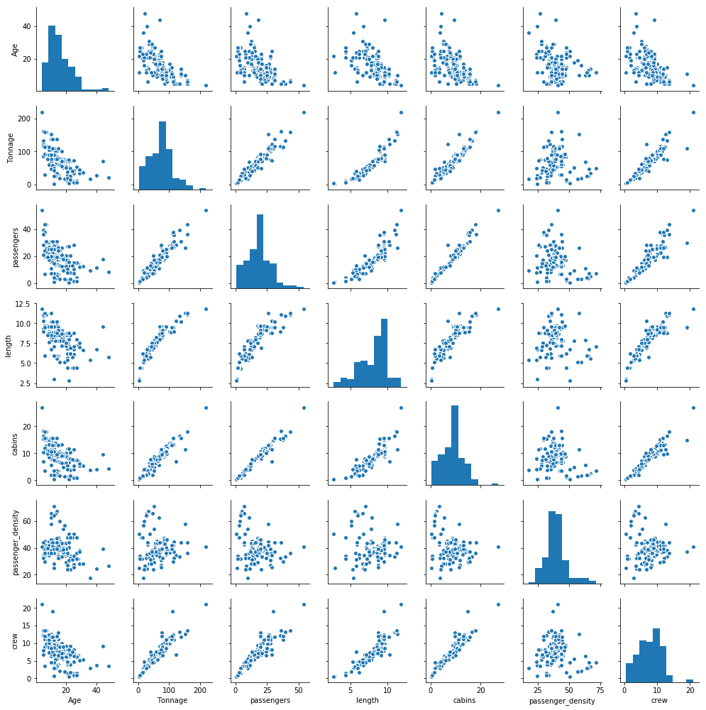
We observe from the pair plots that the target variable ‘crew’ correlates well with 4 predictor variables, namely,’tonnage’, ‘passengers’, ‘length’, and ‘cabins’.
To quantify the degree of correlation, we calculate the covariance matrix.
5. Variable selection for predicting “crew” size
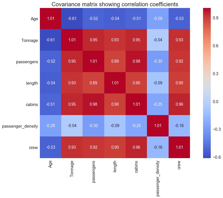
5 (a) Calculation of the covariance matrix
cols = ['Age', 'Tonnage', 'passengers', 'length', 'cabins','passenger_density','crew'] from sklearn.preprocessing import StandardScaler
stdsc = StandardScaler()
X_std = stdsc.fit_transform(df[cols].iloc[:,range(0,7)].values)cov_mat =np.cov(X_std.T)
plt.figure(figsize=(10,10))
sns.set(font_scale=1.5)
hm = sns.heatmap(cov_mat,
                 cbar=True,
                 annot=True,
                 square=True,
                 fmt='.2f',
                 annot_kws={'size': 12},
                 cmap='coolwarm',
                 yticklabels=cols,
                 xticklabels=cols)
plt.title('Covariance matrix showing correlation coefficients', size = 18)
plt.tight_layout()
plt.show()
5 (b) Selecting important variables (columns)
From the covariance matrix plot above, if we assume important features have a correlation coefficient of 0.6 or greater, then we see that the “crew” variable correlates strongly with 4 predictor variables: “tonnage”, “passengers”, “length, and “cabins”.
cols_selected = ['Tonnage', 'passengers', 'length', 'cabins','crew']

df[cols_selected].head()


In summary, we’ve shown how a covariance matrix can be used for variable selection and dimensionality reduction. We’ve reduced the original dimension from 6 to 4.
Other advanced methods for feature selection and dimensionality reduction are Principal Component Analysis (PCA), Linear Discriminant Analysis (LDA), Lasso Regression, and Ridge Regression. Find out more by clicking on the following links:
Towards AI
Towards AI, is the world’s fastest-growing AI community for learning, programming, building and implementing AI.
WRITTEN BY
Physicist, Data Scientist, Educator, Writer. Interests: Data Science, Machine Learning, AI, Python & R, Predictive Analytics, Materials Science, Bioinformatics


No comments:
Post a Comment