Dissecting Dutch Death Statistics with Python, Pandas and Plotly in a Jupyter Notebook
The CBS (the Dutch Centraal Bureau Statistiek) keeps track of many things in The Netherlands. And shares many of its data sets as open data, typically in the form of JSON, CSV or XML files. One of the data sets is published is the one on the number of births and deaths per day. I have taken this data set, ingested and wrangled the data into a Jupyter Notebook and performed some visualization and analysis. This article describes some of my actions and my findings, including attempts to employ Matrix Profile to find repeating patterns or motifs.
TL;DR : Friday is the day of the week with the most deaths; Sunday is a slow day for the grim reaper in our country. December through March is death season and August and September are the quiet period.
The Jupyter Notebook and data sources discussed in this article can be found in this GitHub Repo: https://github.com/lucasjellema/data-analytic-explorations/tree/master/dutch-birth-and-death-data
Preparation: Ingest and Pre-wrangle the data
Our raw data stems from https://opendata.cbs.nl/statline/#/CBS/nl/dataset/70703ned/table?ts=1566653756419. I have downloaded a JSON file with the deaths per day data. Now I am going to explore this file in my Notebook and wrangle it into a Pandas Data Frame that allows visualization and further analysis.


import json import pandas as pd ss = pd.read_json("dutch-births-and-deaths-since-1995.json") ss.head(5)
Data frame ss now contains the contents of the JSON file. The data is yet all that much organized: it consists of individual JSON records that each represent one day — or one month or one year.
I will create additional columns in the data frame — with for each record the date it describes and the actual death count on that date:

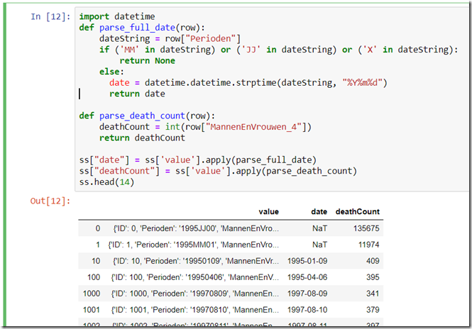
import datetime def parse_full_date(row): dateString = row["Perioden"] if ('MM' in dateString) or ('JJ' in dateString) or ('X' in dateString): return None else: date = datetime.datetime.strptime(dateString, "%Y%m%d") return date def parse_death_count(row): deathCount = int(row["MannenEnVrouwen_4"]) return deathCount ss["date"] = ss['value'].apply(parse_full_date) ss["deathCount"] = ss['value'].apply(parse_death_count) ss.head(14)
Column date is derived by processing each JSON record and parsing the Perioden property that contains the date (or month or year). The date value is a true Python DateTime instead of a string that looks like a date. The deathCount is taken from the property MannenEnVrouwen_4 in the JSON record.
After this step, the data frame has columns date and deathCount that allows us to start the analysis. We do not need the original JSON content any longer, nor do we care for the records that indicate the entire month or year.


# create data frame called data that contains only the data per day data = ss[ss['date'].notnull()][['date','deathCount']]
data.set_index(data["date"],inplace=True)
data.head(4)
Analysis of Daily Death Count
In this Notebook, I make use of Plotly [Express] for creating charts and visualizations:

Let’s look at the evolution of the number of deaths over the years (1995–2017) to see the longer-term trends.


# initialize libraries
import plotly.graph_objs as go
import plotly.express as px from chart_studio.plotly
import plot, iplot from plotly.subplots
import make_subplots
# sample data by year; calculate average daily deathcount
d= data.resample('Y').mean(['deathCount'].to_frame(name='deathCount') d["date"]= d.index
# average daily death count per year (and/or total number of deaths per year)
fig = px.line(d, x="date", y="deathCount", render_mode='svg',labels={'grade_smooth':'gradient'} , title="Average Daily Death Count per Year")
fig.update_layout(yaxis_range=[350,430])
fig.show()
This results in an interactive, zoomable chart with mouse popup — that shows the average number of daily deaths for each year in the period 1995–2017:


The fluctuation is remarkable — 2002 was a far more deadly year than 2008 — and the trend is ominous with the last year (2017) the most deadly of them all.
The conclusion from the overhead plot: there is a substantial fluctuation between years and there seems to be an upward trend (probably correlated with the growth of total population — some 60–70 years prior to the years shown here)
The death count data is a time-series: timestamped records. That means that some powerful operations are at my fingerprints, such as resampling the data with different time granularities. In this case, calculate the yearly sum of deaths and plot those numbers in a bar chart. It will not contain really new information, but it presents the data in a different way:


# sample data by year; calculate average daily deathcount
d= data.copy().resample('Y').sum()['deathCount'].to_frame(name='deathCount')
d["date"]= d.index
fig = px.bar(d , x="date", y="deathCount" ,title="Total Number of Deaths per Year" , range_y=[125000,155000] , barmode="group" )
fig.show()
And the resulting chart:


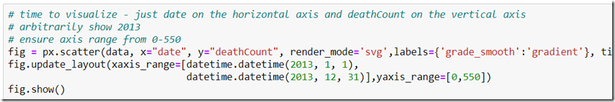
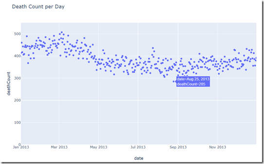
The next scatter plot shows all number of deaths on day values for a randomly chosen period; the fluctuation from day to day is of course quite substantial. The seasonal fluctuation still shows up.
# arbitrarily show 2013
# ensure axis range from 0-550
fig = px.scatter(data, x="date", y="deathCount", render_mode='svg',labels={'grade_smooth':'gradient'}, title="Death Count per Day")
fig.update_layout(xaxis_range=[datetime.datetime(2013, 1, 1), datetime.datetime(2013, 12, 31)],yaxis_range=[0,550])
fig.show()


The next chart shows the daily average number of deaths calculated for each month:
# create a new data frame with the daily average death count calculated for each month; this shows us how the daily average changes month by month
d= data.copy().resample('M').mean()['deathCount'].to_frame(name='deathCount')
d["date"]= d.index
fig = px.scatter(d, x="date", y="deathCount", render_mode='svg',labels={'grade_smooth':'gradient'} , title="Average Daily Death Count (per month)")
fig.update_layout(xaxis_range=[datetime.datetime(2005, 1, 1), datetime.datetime(2017, 12, 31)],yaxis_range=[0,550])
fig.show()


And the chart:


Day of the Week
One question that I am wondering about: is the number of deaths equally distributed over the days of the week. A quick, high-level exploration makes clear that there is a substantial difference between the days of the week:
cats = [ 'Monday', 'Tuesday', 'Wednesday', 'Thursday', 'Friday', 'Saturday', 'Sunday']
# create a new data frame with the death counts grouped by day of the week
# reindex is used to order the week days in a logical order (learned from https://stackoverflow.com/questions/47741400/pandas-dataframe-group-and-sort-by-weekday)
df_weekday = data.copy().groupby(data['date'].dt.weekday_name).mean().reindex(cats)
df_weekday

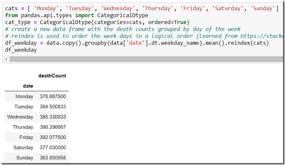
In over 20 years of data, the difference between Friday and Sunday is almost 30 — or close to 8%. That is a lot — and has to be meaningful.
A quick bar chart is easily created:
df_weekday['weekday'] = df_weekday.index
# draw barchart
fig = px.bar(df_weekday , x="weekday", y="deathCount" , range_y=[350,400] , barmode="group" )
fig.update_layout( title=go.layout.Title( text="Bar Chart with Number of Deaths per Weekday" ))
fig.show()


And confirms our finding visually:


To make sure we are looking at a consistent picture — we will normalize the data. What I will do in order to achieve this is to calculate an index value for each date — by dividing the death count on that date by the average death count in the seven day period that this date is in the middle of. Dates with a high death count will have an index value of 1.05 or even higher and ‘slow’ days will have an index under 1, perhaps even under 0.95. Regardless of the seasonal and multi-year trends in death count, this allows us to compare, aggregate and track the performance of each day of the week.
The code for this [may look a little bit intimidating at first]:
d = data.copy()
d.loc[:,'7dayavg'] = d.loc[:,'deathCount'].rolling(window=7,center=True).mean()
d.loc[:,'relativeWeeklyDayCount'] = d.loc[:,'deathCount']/d.loc[:,'7dayavg'] cats = [ 'Monday', 'Tuesday', 'Wednesday', 'Thursday', 'Friday', 'Saturday', 'Sunday'] df_weekday = d.copy().groupby(d['date'].dt.weekday_name).mean().reindex(cats)
df_weekday['weekday'] = df_weekday.index
# draw barchart
fig = px.bar(df_weekday , x="weekday", y="relativeWeeklyDayCount" , range_y=[0.95,1.03] , barmode="group" )
fig.update_layout( title=go.layout.Title( text="Bar Chart with Relative Number of Deaths per Weekday" ))
fig.show()


The 2nd and 3rd line is where the daily death count index is calculated; first the rolling average over 7 days and subsequently the division of the daily death count by the rolling average.
The resulting bar chart confirms our finding regarding days of the week:


Over the full period of our data set — more than 20 years worth of data, there is close to 0.08 difference between Friday and Sunday.
I want to inspect next how the index value for each week day has evolved through the 20 years. Was Sunday always the day of the week with the smallest number of deaths? Has Friday consistently been the day with the highest number of deaths?
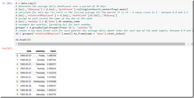
I have calculated the mean index per weekday over periods of one quarter; for each quarter, I have taken the average index value for each day of the week. And these average index values were subsequently plotted in a line chart.
d = data.copy()
# determine the average daily deathcount over a period of 30 days
d.loc[:,'30dayavg'] = d.loc[:,'deathCount'].rolling(window=30,center=True).mean()
# calculate for each day its ratio vs the rolling average for the period it is in - a value close to 1 - between 0.9 and 1.1
d.loc[:,'relative30DayCount'] = d.loc[:,'deathCount']/d.loc[:,'30dayavg']
# assign to each record the name of the day of the week
d.loc[:,'weekday'] = d['date'].dt.weekday_name
# resample per quarter, (grouping by) for each weekday
grouper = d.groupby([pd.Grouper(freq='1Q'), 'weekday'])
# create a new data frame with for each Quarter the average daily death index for each day of the week (again, between 0.9 and 1.1)
d2 = grouper['relative30DayCount'].mean().to_frame(name = 'mean').reset_index()
d2.head(10)

Let’s now show the line chart:
fig = px.line(d2, x="date", y="mean", color="weekday" ,render_mode='svg',labels={'grade_smooth':'gradient'} , title="Average Daily Death Count Index per Quarter")
fig.show()

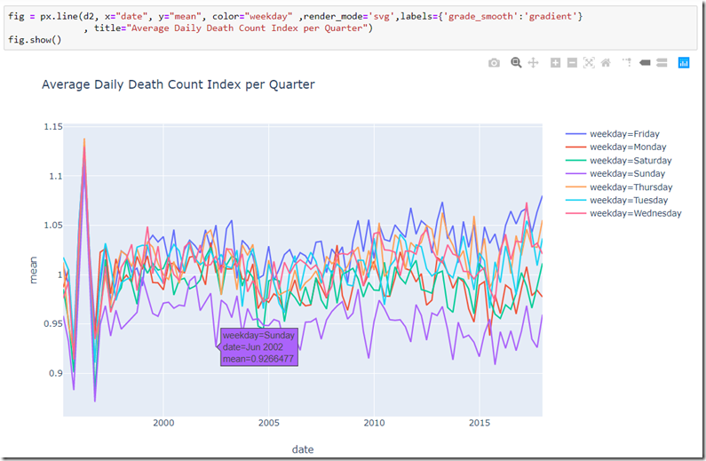
This chart shows how Sunday has been the day of the week with the lowest death count for almost every quarter in our data set. It would seem that Friday is the day with the highest number of deaths for most quarters. We see some peaks on Thursday.
The second quarter of 2002 (as well as Q3 2009) shows an especially deep trough for Sunday and a substantial peak for Friday. Q1 2013 shows Friday at its worst.
Note: I am not sure yet what strange phenomenon causes the wild peak for all weekday in Q1 1996. Something is quite off with the data it would seem.
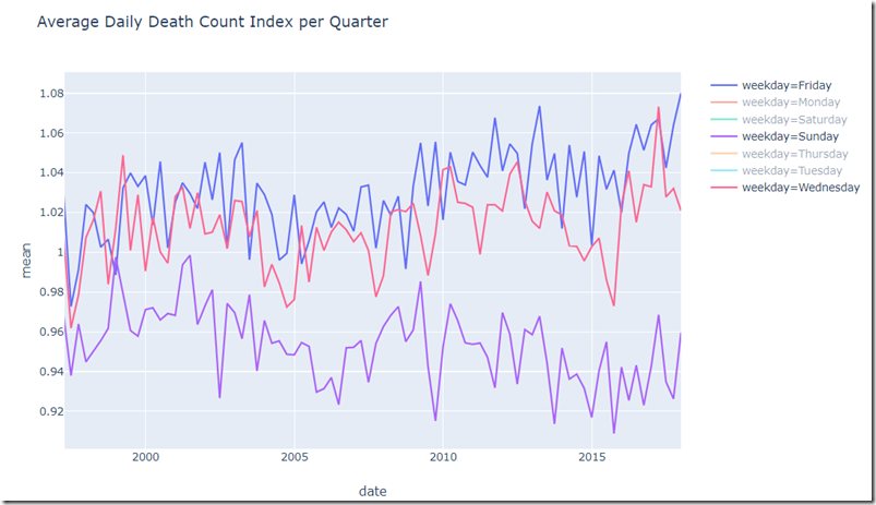
The PlotLy line chart has built-in functionality for zooming and filtering selected series from the chart, allowing this clear picture of just Friday, Wednesday and Sunday. The gap between Sunday and Friday is quite consistent. There seems to be a small trend upwards for Friday (in other words: the Friday effect becomes more pronounced) and downwards for Sunday.

The Deadly Season — Month of Year
Another question I have: is the number of deaths equally distributed over the months of the year. Spoiler alert: no, it is not. The dead of winter is quite literally that.
The quick inspection: data is grouped by month of the year and the average is calculated for each month (for all days that fall in the same month of the year, regardless of the year)
# create a new data frame with the death counts grouped by month
df_month = data.copy().groupby(data['date'].dt.month).mean()
import calendar
df_month['month'] = df_month.index
df_month['month_name'] = df_month['month'].apply(lambda monthindex:calendar.month_name[monthindex])
# draw barchart
fig = px.bar(df_month , x="month_name", y="deathCount" , range_y=[320,430] , barmode="group" )
fig.update_layout( title=go.layout.Title( text="Bar Chart with Number of Average Daily Death Count per Month" ))
fig.show()


The bar chart reveals how the death count varies through the months of the year. The range is quite wide — from an average of 352 in August to a yearly high in January of 427. The difference between these months is 75 or more than 20%. It will be clear when the undertakers and funeral homes can best plan their vacation.


The powerful resample option can be used to very quickly create a data set with mean death count per month for all months in our data set.
m = data.copy().resample('M').mean()
m['monthstart'] = m.index
# draw barchart
fig = px.bar(m , x="monthstart", y="deathCount" #, range_y=[0,4000] , barmode="group" )
fig.update_layout( title=go.layout.Title( text="Bar Chart with Daily Average Death Count per Month" ))
fig.show()


The resulting chart shows that the average daily death count ranges with the months from a daily average of 510 in chilly January 2017 to only 330 in care free August of 2009. A huge spread!


Resources
The Jupyter Notebook and data sources discussed in this article can be found in this GitHub Repo: https://github.com/lucasjellema/data-analytic-explorations/tree/master/dutch-birth-and-death-data
Our raw data stems from https://opendata.cbs.nl/statline/#/CBS/nl/dataset/70703ned/table?ts=1566653756419.
Originally published at https://technology.amis.nl on October 10, 2019.
Oracle Developers
Aggregation of articles from Oracle & partners engineers, Groundbreaker ambassadors & the developer community on all things Oracle Cloud and its technologies. The views expressed are those of authors solely and do not necessarily reflect Oracle's. Contact @jimgris or @brhubart
WRITTEN BY
Lucas Jellema is solution architect and CTO at AMIS, The Netherlands. He is Oracle ACE Director, Groundbreaker Ambassador, JavaOne Rockstar and programmer


No comments:
Post a Comment