Plant diseases can be detected by leveraging the power of Deep Learning.

Inthis article, I’m going to explain how we can use the Deep Learning Models to detect and classify the diseases of plants and guide the farmers through videos and give instant remedies to overcome the loss of plants and fields. At first, we have to understand
- What is the cause and how to overcome the cause?
2. What are the benefits of doing this?
3. Can we solve this problem with “Deep Learning technology”?
4. In Deep Learning “which Algorithm” is used to address this problem ? and how to do that ?.
NOTE: I did it only for Tomato and Potato plants. you can do it for other plants by collecting data of that plant.
It also deployed to Web App. Check out below Link.
1. The Cause And Introduction.
Since the past days and in the present too, farmers usually detect the crop diseases with their naked eye which makes them take tough decisions on which fertilisers to use. It requires detailed knowledge the types of diseases and lot of experience needed to make sure the actual disease detection. Some of the diseases look almost similar to farmers often leaves them confused. Look at the below image for more understanding.


They look the same and almost similar. In case the farmer makes wrong predictions and uses the wrong fertilizers or more than the normal dose (or) threshold or Limit (every plant has some threshold fertilizers spraying to be followed), it will mess up the whole plant (or) soil and cause enough damage to plant and fields.


So, How to prevent this from happening?
To prevent this situation we need better and perfect guidance on which fertilizers to use, to make the correct identification of diseases, and the ability to distinguish between two or more similar types of diseases in visuals.
This is where Artificial Neural Networks comes handy. In short ANN
2. What is ANN?
Artificial Neural Nets are computational model based on structure of biological neural nets designed to mimic the actual behaviour of a biological neural network which are present in our brain.

Sowe can assign some stuff to it, it gets our job done. ANN helps us to make the correct identification of disease and also guiding the right quantity of fertilizers.
Only a single ANN can’t get our job done. So, we make a bunch of them stacking one on other forming a layer which we can make multiple layers in between input layer(where weights and data are given) and output layer(result) those multiple layers called Hidden layers and it then makes a Deep Neural Network and the study of it called Deep Learning.
2.1 How does it looks like The Deep Neural Network.

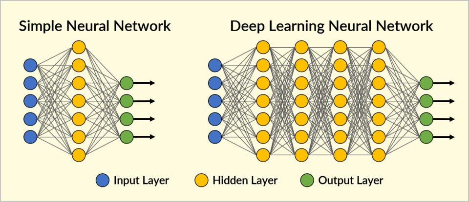
Simple Neural Nets are good at learning the weights with one hidden layer which is in between the input and output layer. But, it’s not good at complex feature learning.
On another hand Deep Learning Neural Nets, the series of layers between input and output layer are called hidden layers that can perform identification of features and creating new series of features from data, just as our brain. The more layers we push into the more features it will learn and perform complex operations. The output layer combines all features and makes predictions.
Therefore, Simple Neural Nets are used for simple tasks and bulk data isn’t required to train itself. whereas in Deep learning Neural Network can be expensive and require massive data sets to train itself on. I’m not gonna discuss this topic cause it goes beyond this article.
IF you are absolute beginner to Deep Learning concept below link would help to get all basics.
2.2 What type of Deep Learning Model is best for this scenario??
There you go Convolutional Neural Network(CNN or Conv Nets). It is well known for its widely used in applications of image and video recognition and also in recommender systems and Natural Language Processing(NLP). However, convolutional is more efficient because it reduces the number of parameters which makes different from other deep learning models.


To keep it simple I will explain only the brief understanding of this model and the steps that are used in building Convolutional Neural Network.
Main Steps to build a CNN (or) Conv net:
- Convolution Operation
- ReLU Layer (Rectified Linear Unit)
- Pooling Layer (Max Pooling)
- Flattening
- Fully Connected Layer
Start Writing Code.
1. Convolution is the first layer to extract features from the input image and it learns the relationship between features using kernel or filters with input images.
2. ReLU Layer: ReLU stands for the Rectified Linear Unit for a non-linear operation. The output is ƒ(x) = max(0,x). we use this because to introduce the non-linearity to CNN.
3. Pooling Layer: it is used to reduce the number of parameters by downsampling and retain only the valuable information to process further. There are types of Pooling:
- Max Pooling (Choose this).
- Average and Sum pooling.
4. Flattening: we flatten our entire matrix into a vector like a vertical one. so, that it will be passed to the input layer.
5. Fully Connected Layer: we pass our flatten vector into input Layer .we combined these features to create a model. Finally, we have an activation function such as softmax or sigmoid to classify the outputs.
3. Done understanding CNN Operations. What next??
- Gathering Data (Images)
Gather the data sets as many as you can with Images affected by diseases and also which are healthy. you should require bulk data.


2. Building CNN.
Build CNN using some popularly used open-source Libraries for the development of AI, Machine Learning and also Deep Learning.


3. Choose Any Cloud-Based Data Science IDE’s.
It is good to train models in the cloud as it requires massive computation power our normal machines laptops and the computer won’t sustain. If you have a good GPU config laptop you can train in your local machine. I choose Google colab you can choose whatever cloud you like.
Google Colab:
Google colab is a free cloud service which offers free GPU(12Gb ram). It’s a hassle free and fastest way to train our model no need to installation of any libraries on our machine. it works completely on cloud. It comes pre-installed with all dependencies.


Sign-in to colab and create a new python notebook(ipynb) switch to GPU mode and start writing code.
4. Start Writing Code.
Data should be stored in Google drive before writing code.
Source Code can be found here My GitHub link .
Step 1: Mount data from google drive.
from google.colab import drive
drive.mount(‘/content/your path’)
Step 2: Import Libraries.
# Import Libraries
import os
import glob
import matplotlib.pyplot as plt
import numpy as np# Keras API
import keras
from keras.models import Sequential
from keras.layers import Dense,Dropout,Flatten
from keras.layers import Conv2D,MaxPooling2D,Activation,AveragePooling2D,BatchNormalization
from keras.preprocessing.image import ImageDataGenerator
Step 3: Load train and test data into separate variables.
# My data is in google drive.
train_dir ="drive/My Drive/train_set/"
test_dir="drive/My Drive/test_data/"
Step 4: Function to Get count of images in train and test data.
# function to get count of images
def get_files(directory):
  if not os.path.exists(directory):
    return 0
  count=0
  for current_path,dirs,files in os.walk(directory):
    for dr in dirs:
      count+= len(glob.glob(os.path.join(current_path,dr+"/*")))
  return count
Step 5: View number of images in each.
train_samples =get_files(train_dir)
num_classes=len(glob.glob(train_dir+"/*"))
test_samples=get_files(test_dir)
print(num_classes,"Classes")
print(train_samples,"Train images")
print(test_samples,"Test images")


- 12 Classes == 12 types of diseases images are collected.
- 14955 Train Images
- 432 Test images (i took only a few images to test mistakenly).
- For prediction, I took only a few samples from unseen data. we can evaluate using validation data which is part of train data.
Step 6: Pre-processing our raw data into usable format.
# Pre-processing data with parameters.
train_datagen=ImageDataGenerator(rescale=1./255,
                                   shear_range=0.2,
                                   zoom_range=0.2,
                                   horizontal_flip=True)
test_datagen=ImageDataGenerator(rescale=1./255)
- Rescaling image values between (0 –1) called normalization.
- whatever pre-processing you do with the train it should be done to test parallelly.
- All these parameters are stored in the variable “train_datagen and test_datagen”.
Step 7: Generating augmented data from train and test directories.
# set height and width and color of input image.
img_width,img_height =256,256
input_shape=(img_width,img_height,3)
batch_size =32train_generator =train_datagen.flow_from_directory(train_dir,
                                target_size=(img_width,img_height),                                                    batch_size=batch_size)
test_generator=test_datagen.flow_from_directory(test_dir,shuffle=True,target_size=(img_width,img_height),                                               batch_size=batch_size)
- Takes the path to a directory, and generates batches of augmented data. Yields batches indefinitely, in an infinite loop.
- Batch Size refers to the number of training examples utilized in one iteration.


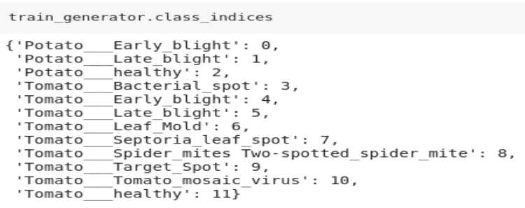
Step 8: Get 12 Diseases Names/classes.
# The name of the 12 diseases.
train_generator.class_indices

Step 9: Building CNN model
# CNN building.
model = Sequential()
model.add(Conv2D(32, (5, 5),input_shape=input_shape,activation='relu'))
model.add(MaxPooling2D(pool_size=(3, 3)))
model.add(Conv2D(32, (3, 3),activation='relu'))
model.add(MaxPooling2D(pool_size=(2, 2)))
model.add(Conv2D(64, (3, 3),activation='relu'))
model.add(MaxPooling2D(pool_size=(2, 2)))
model.add(Flatten())
model.add(Dense(512,activation='relu'))
model.add(Dropout(0.25))
model.add(Dense(128,activation='relu'))
model.add(Dense(num_classes,activation='softmax'))
model.summary()


CNN shrinks the parameters and learns features and stores valuable information output shape is decreasing after every layer. Can we see the output of every layer? Yes!! We can.
Step 10: Visualisation of images after every layer.
from keras.preprocessing import image
import numpy as np
img1 = image.load_img('/content/drive/My Drive/Train_d/Tomato___Early_blight/Tomato___Early_blight/
(100).JPG')
plt.imshow(img1);
#preprocess image
img1 = image.load_img('/content/drive/MyDrive/Train_d/
Tomato___Early_blight/Tomato___Early_blight(100).JPG', target_size=(256, 256))
img = image.img_to_array(img1)
img = img/255
img = np.expand_dims(img, axis=0)
- Take a sample image from the train data set and visualize the output after every layer.
- NOTE: Pre-processing is needed for the new sample image.
from keras.models import Model
conv2d_1_output = Model(inputs=model.input, outputs=model.get_layer('conv2d_1').output)
max_pooling2d_1_output = Model(inputs=model.input,outputs=model.get_layer('max_pooling2d_1').output)conv2d_2_output=Model(inputs=model.input,outputs=model.get_layer('conv2d_2').output)
max_pooling2d_2_output=Model(inputs=model.input,outputs=model.get_layer('max_pooling2d_2').output)conv2d_3_output=Model(inputs=model.input,outputs=model.get_layer('conv2d_3').output)
max_pooling2d_3_output=Model(inputs=model.input,outputs=model.get_layer('max_pooling2d_3').output)flatten_1_output=Model(inputs=model.input,outputs=model.get_layer('flatten_1').output)conv2d_1_features = conv2d_1_output.predict(img)
max_pooling2d_1_features = max_pooling2d_1_output.predict(img)
conv2d_2_features = conv2d_2_output.predict(img)
max_pooling2d_2_features = max_pooling2d_2_output.predict(img)
conv2d_3_features = conv2d_3_output.predict(img)
max_pooling2d_3_features = max_pooling2d_3_output.predict(img)
flatten_1_features = flatten_1_output.predict(img)


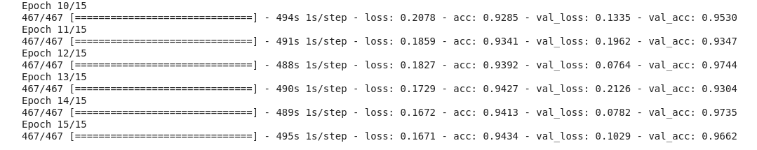
Step 11. Start Training CNN with Parameters.
validation_generator = train_datagen.flow_from_directory(
                       train_dir, # same directory as training data
                       target_size=(img_height, img_width),
                       batch_size=batch_size)opt=keras.optimizers.Adam(lr=0.001)
model.compile(optimizer=opt,loss='categorical_crossentropy',metrics=['accuracy'])
train=model.fit_generator(train_generator,nb_epoch=20,                             steps_per_epoch=train_generator.samples//batch_size,                        validation_data=validation_generator,nb_val_samples=validation_generator.samples // batch_size,verbose=1)
- Adam optimizer is used with learning rate=0.001
- Loss function categorical_crossentropy is used for our Multi-class classification problem. Metrics is “ accuracy”.
- Fit_generator is used to train the CNN model. Using the validation data parameter for fine-tuning the model.

Step 12: Saving Model weights.
- Saving model weights to prevent from re-training of the model.
# Save model
from keras.models import load_model
model.save('crop.h5')
Step 13: Load Model from saved weights.
# Loading model and predict.
from keras.models import load_model
model=load_model('crop.h5')# Mention name of the disease into list.
Classes = ["Potato___Early_blight","Potato___Late_blight","Potato___healthy","Tomato___Bacterial_spot","Tomato___Early_blight","Tomato___Late_blight","Tomato___Leaf_Mold","Tomato___Septoria_leaf_spot","Tomato___Spider_mites Two-spotted_spider_mite","Tomato___Target_Spot","Tomato___Tomato_mosaic_virus","Tomato___healthy"]
- Mentioning the name because our output is in numeric format. We cast it into strings.
Step 14: Predictions
import numpy as np
import matplotlib.pyplot as plt# Pre-Processing test data same as train data.
img_width=256
img_height=256
model.compile(optimizer='adam',loss='categorical_crossentropy',metrics=['accuracy'])from keras.preprocessing import imagedef prepare(img_path):
    img = image.load_img(img_path, target_size=(256, 256))
    x = image.img_to_array(img)
    x = x/255
    return np.expand_dims(x, axis=0)


result = model.predict_classes([prepare('/content/drive/My Drive/Test_d/Tomato_BacterialSpot/Tomato___Bacterial_spot (901).JPG')])
disease=image.load_img('/content/drive/My Drive/Test_d/Tomato_BacterialSpot/Tomato___Bacterial_spot (901).JPG')
plt.imshow(disease)
print (Classes[int(result)])
- we need to preprocess our image to pass in a model to predict
- First, we resize the image ===> image(150,150)
- convert image to array by this it will add channels===>image(150,150,3) RGB
- Tensorflow works with batches of images we need to specify image samples===>(1,150,150,3).
- Predict_classes help to predict the new image belongs to the respective class.


Final Step: Convert Model into “tflite”.
from tensorflow.contrib import lite
converter = lite.TFLiteConverter.from_keras_model_file( 'crop.h5' )
model = converter.convert()
file = open( 'output.tflite' , 'wb' )
file.write( model )
- To make our model communicate with App we have to convert into the TensorFlow lite version, tflite is made for mobile Versions.
- So, you can build or create a mobile app and make the app communicate with the model.
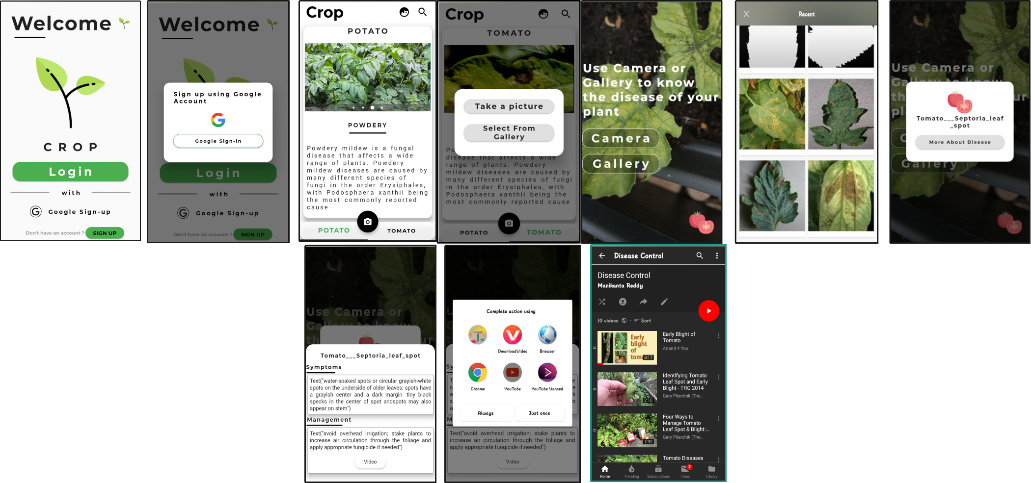
You can use the Google flutter framework to build apps with beautiful UI’s.


Before moving on into App part, you need setup the installation of flutter environment into your machine from Official website.
Open up flutter editor either Android studio or visual studio as you wish to code.


Create a new flutter Project and make a folder in project files drop “output.tflite” file into assets folder into our flutter project .Below name is changed but tflite file is same.

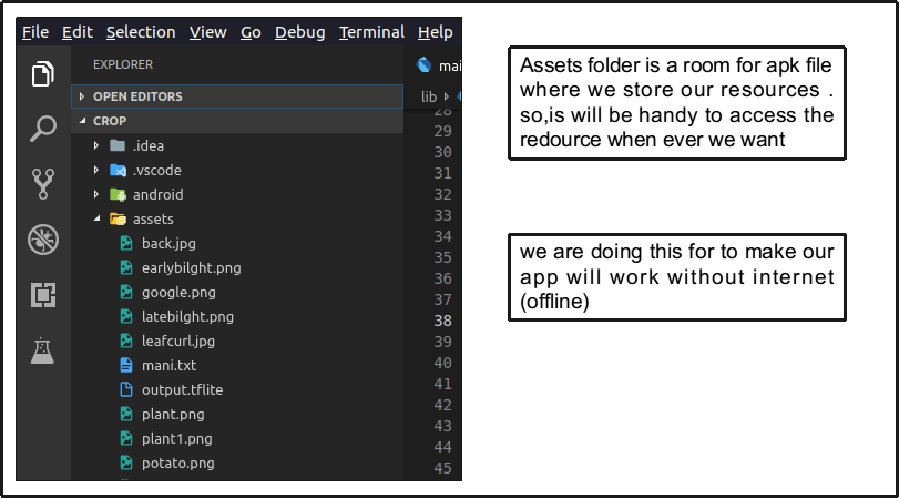
The App User Interface can be of your choice, you can make one by learning flutter or just use my flutter app interface. It can be found in my Github.
Once you are done with dropping “output.tflite” in the assets folder, start running the app in the emulator and test model with some pictures that are from the test folder and also with real images that are unseen by the model before.
Conclusion:
Plant Diseases are major food threats that should have to overcome before it leads to further loss of the entire field. But, often framers unable to distinguish between similar symptoms but ace different diseases. This will mislead to wrong or overdosage of fertilizers. Here, we employ Convolutional Neural Network(CNN) multiple layers of ANN called Deep Learning Algorithms to reduce this loss and guide farmers with video lessons. This can be done through mobile App “Not all farmers but some do use it.”
I hope the above stuff would useful for everyone reading this article. I will surely come up with topics related to Data Science, ML, and DL. Happy Learning :)


2 comments:
source code for the flutter mobile app please
Useful blog, keep sharing with us.
How Does Google Flutter Work
Why Google Flutter
Post a Comment