Lessons Learned Using Google Cloud BigQuery ML
Start-to-finish ML demo using German Credit Data


Motivation
A new buzzword I hear often is “democratize AI for the masses”. Usually what follows is a suggested Cloud Machine Learning tool. The umbrella term for these tools seems to be AML, or Automatic Machine Learning. As a Data Scientist myself, I was curious to investigate these tools. Some questions going through my mind: What can AML really do? Can I use these tools in my usual modeling workflow? If so, how and for what benefits? Will my usefulness as a human with ML skills go away soon?
My plan is to demo the most popular AML tools, using the same “real” dataset each time, comparing run time, fit metrics, steps how I would productionize, and some UI screenshots.
In my work recently, I needed to build and deploy financial fraud detection models. I can’t use proprietary data in a public blog post, so I’m going to use the well-known public dataset German Credit Data. Note the cost matrix is 5 DM per False Negative and 1 DM per False Positive. Even though the data is small, I’ll walk through all the same techniques I’d use for real data. Code for all the demos will be on my github.
My plan is to cover these popular AML tools:
- Part 1 (this post): Google’s Big Query on Google Cloud Platform (GCP).
Parts 2, 3, 4 coming soon hopefully(!) :
- Part 2: Tensorflow 2.0 using Keras on Google Cloud Platform (GCP).
- Part 3: Databricks MLFlow on AWS using Scala
- Part 4: H2O’s AutoML, and Cisco’s Kubeflow Hyperparameter Tuning. Focus on algorithm comparison and hyperparameter selection.
BigQuery ML — Step 1) create the data
Let’s get started. Google’s BigQuery offers a number of free public datasets. You can search for them here. I did not see any credit data, so I used Google’s BigQuery sandbox to upload mine. BigQuery sandbox is Google’s GCP free tier cloud SQL database. It’s free but your data only lasts 60 days at a time.
For all the Google Cloud tools you have to first create a Google Cloud account and a project. Next, assign Sandbox resource to the project follow these instructions. Now go to https://console.cloud.google.com/bigquery, this is the Web UI. Next, pin your Sandbox-enabled project (see screenshot below left). Next, load your data using the Web UI. I called my table “allData”.
The German Credit Data is a very small dataset, only 998 rows. Normally, best practice is to split your data into train/valid/test, but since this is so small, I’m going to split into 80/20 train/test and use cross-validation technique to stretch out the train into train/valid. Note: I created a fake `uniqueID` column (see screenshot below right), to help with the random splitting.


Here’s the SQL I used to create “trainData” and “testData” as randomly sampled rows from “allData”.
CREATE TABLE cbergman.germanCreditData.testData AS
SELECT *
FROM `cbergman.germanCreditData.allData`
WHERE MOD(ABS(FARM_FINGERPRINT(CAST(uniqueID AS STRING))), 5) = 0;

CREATE OR REPLACE TABLE cbergman.germanCreditData.trainData AS
SELECT *
FROM `cbergman.germanCreditData.allData`
WHERE NOT uniqueID IN (
  SELECT DISTINCT uniqueID FROM `cbergman.germanCreditData.testData`
);
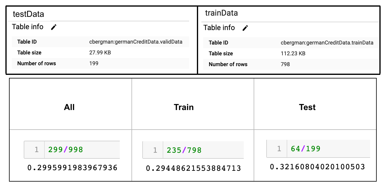
Now I have my tables loaded in BigQuery with 199 and 798 rows respectively. Check that the random sample did the right thing:
SELECT count (distinct uniqueID)
FROM `cbergman.germanCreditData.allData`
where response = 2;

# repeat for train, test data...
See bottom row below, I end up with ratios of negative (response=1) to positive (response=2) as 30%, 29%, 32% per All/Train/Test datasets, which looks like a good sampling:

BigQuery ML — Step 2) train a ML model
At the time of writing this, the API gives you have a choice of 3 algorithms: Regression, Logistic Regression, or K-Nearest Neighbors. Before creating your model, usually you have to: 1) make sure the business objectives are clear: “Try to catch the most fraud money automatically you can”. At my work, fraud money is further split up into types of fraud e.g. 3rd party. 2) Next, you usually have to translate that to math model algorithm: in this case classification so choose API method Logistic Regression. 3) Next, you define the loss function, which in a real company is tricky since one department might say new users are more important; while the risk department says all fraud is more important. In one company I worked at, for example, they could not agree on a single loss metric. However, this problem is solved here, the creators of this public data gave a cost matrix 5 DM per False Negative and 1 DM per False Positive.
With business definitions done, see screenshot below, how you might train a base model by running a SQL query from the Query editor. Under the Training details, the Loss per iteration is decreasing, which is what we expect; and since this is a logistic regression, the loss is log loss.

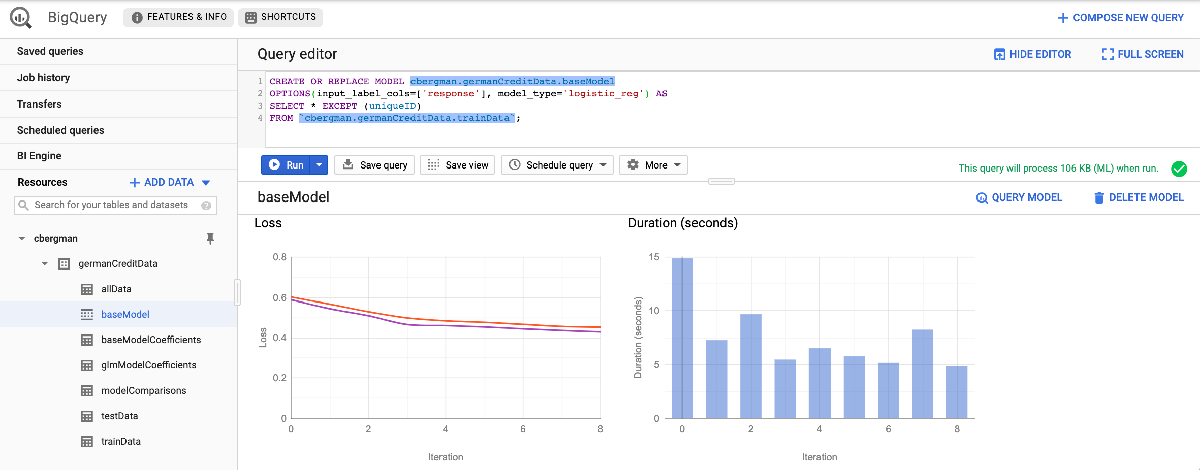
Below is the SQL to create the model and examine model fit on train and test data.
# Create the base model
CREATE OR REPLACE MODEL cbergman.germanCreditData.baseModel OPTIONS(input_label_cols=['response'], model_type='logistic_reg') AS
SELECT * EXCEPT (uniqueID)
FROM `cbergman.germanCreditData.trainData`;# Model fit on train data
SELECT *
FROM ML.EVALUATE(MODEL `cbergman.germanCreditData.baseModel`,
(
  SELECT * EXCEPT (uniqueID)
  FROM `cbergman.germanCreditData.trainData`);# Model fit on test data
SELECT *
FROM ML.EVALUATE(MODEL `cbergman.germanCreditData.baseModel`,
(
  SELECT * EXCEPT (uniqueID)
  FROM `cbergman.germanCreditData.testData`);# To view your linear beta-values
SELECT * from ML.WEIGHTS(MODEL cbergman.germanCreditData.baseModel);# To get test data confusion matrix
SELECT *
FROM ML.CONFUSION_MATRIX(MODEL `cbergman.germanCreditData.baseModel`,
(
  SELECT* EXCEPT (uniqueID)
  FROM `cbergman.germanCreditData.testData`);
My baseline logistic regression trained in 1 min 36 sec, ran on test in 0.7 sec, with train ROC_AUC = 0.84, test ROC_AUC = 0.75, Recall = 0.41 and cost 38 * 5 + 12 = 202 DM.
I noticed the train AUC was 0.84, so some slight overfitting happened. I’m not surprised since all the variables were used (SELECT *), and logistic regression is a linear model, which requires all the inputs to be independent. Part of creating a baseline linear model is cleaning up collinear inputs. I know how to do this in Python, so that’s where I’ll turn later.
Meantime, we can inspect and save the beta-values for coefficients of the logistic regression model, and confusion matrix on the hold-out and performance metrics on the hold-out validation data. Note: unless you specify otherwise, the default threshold will be 0.5. I calculated the default confusion matrix normalized and unnormalized, and saved them in a modelComparisons table (I backed up the coefficients and perf stats tables in Google Sheets, very easy menu nav in the WebUI, since I’m conscious my free data will disappear in 60 days).
Step 3) Feature Engineering
What follows is “secret sauce” from an experienced practitioner how to get a better model. I’m switching now to Jupyter notebook, since I know how to clean up collinear inputs in Python. I first check correlations for the numeric columns. Below, highlighted red box on right, we see Amount and Duration are correlated 63%. This makes sense, amount and duration of a loan both probably increase together, we can confirm this in the pair-plots (smaller red-outlined plots on left). Below, bottom row shows all the numeric variables pair-plotted against response 1 or 2, visibly nothing looks related. I’ll drop the Duration field.


Quite a few of the variables are String categories. I’d like to do a VIF-analysis of the String variables, to do that I’ve implemented in Python the Informational R package, sometimes called “Weight-of-Evidence using Information Value”. The idea of the Informational or WOE binning is to go beyond adding new variables via One-Hot-Encoding, to actually bin and number the categories in ascending linear order with the response variable. E.g. if you have variable “Vehicles” with categories “car”, “boat”, “truck” then the conversion to numbers 1, 2, 3 for example representing car, boat, truck will be chosen to align with the response variable. Actually, you won’t have 1, 2, 3 but an informationally-aligned numbering to your response.
After I do the informational-linear-binning, I can calculate VIFs and re-run correlations, see results below.


VIF factors are above left. Interestingly, job and telephone look closely related in terms of variance explanation. Maybe unemployed/non-residents are less likely to have telephones? Another variance-coverage pair looks like sex is related to other_debtor. Hmm, this suggests married/divorced Females are more likely to have a co-applicant. Job and telephone are at the top of redundant variance explainers, so based on VIFs, I’m going to drop the telephone field.
Correlations, above right, look a lot cleaner now. The only concern might be n_credits is 40% correlated with credit_his and property is 36% correlated with housing. Based on correlations, I’ll drop n_credits and property.
In summary, I dropped duration, n_credits, property, and telephone fields and added log transforms to numeric feature calcs. My original 21 fields have now become 64 all-numeric fields. Mostly due to adding numeric transformations: mean, median, max, min, and log-transforms. My category fields-count remained the same due to using Informational binning instead of One Hot Encoding.
Next, I’ll run all my transformed variables through Elastic Net Lasso variable selection. (Note: if someone were to ask me who is my ML Hero, my first response would be Trevor Hastie!). Usually with k-fold cross-validation, k=10 folds is best practice. The trade-off more folds is you get more runs to average over (k=10) versus samples per fold N/k. Since my data is so small I chose k=4-fold cross-validation so that I’d have 199 samples per fold. I end up with the model below.

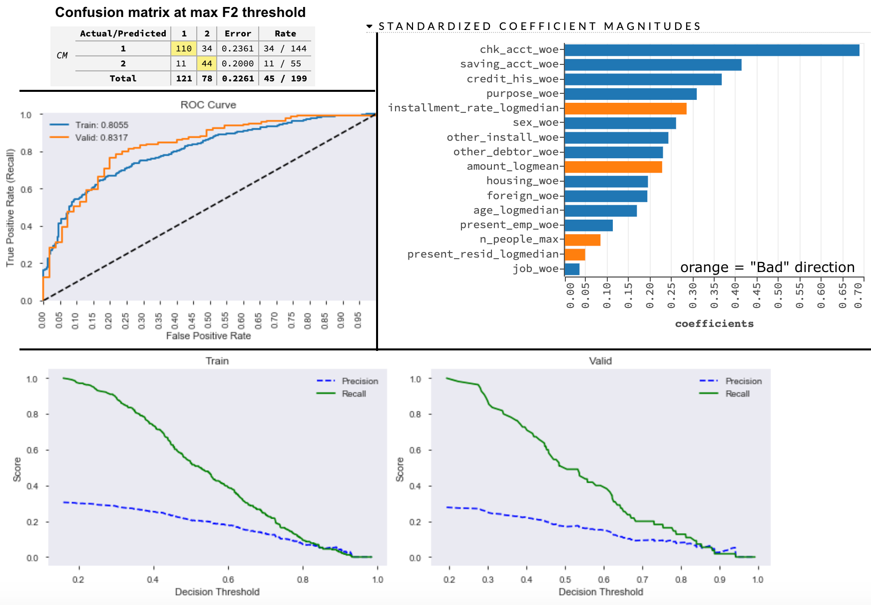
Above middle-left, the ROC curves look reasonably aligned. Above bottom, both train and valid Precision-Recall curves appear to intersect around threshold = 0.9 which shows reassuring consistency. Above top-right, the largest coefficient was for “Checking Account”. I can look into the Information binning to see ordering A11 (neg balance), A12 (< 200DM), A13 (>= 200DM), A14 (no checking acct) in ascending order for predicting getting a loan. We also notice amount and duration were negatively related to getting a loan. Curiously, the “job skill level” didn’t seem to matter so much for predicting “Good” or “Bad” loan outcomes, for “unskilled — non-resident” vs “unskilled — resident” vs “management/officer”. Maybe this all makes sense, I’d probably want to check this with a domain expert.
For now, I’m sticking with this logistic regression model which trained in 3.6 sec, ran on test data in 0.5 sec with training ROC_AUC = 0.81 and test ROC_AUC = 0.83 with cost 11 * 5 + 34 = 89 DM. We’ve saved 50% over the base model cost!! And used fewer variables, with less variance between training and validation. This model is clearly an improvement, and if we were competing, we’d be in the Kaggle Leaderboard, since top score has test AUC around 78%. Nice.
After feature engineering, the next steps are usually:
1) algorithm comparisons
2) hyperparameter tuning
3) threshold tuning
1) algorithm comparisons
2) hyperparameter tuning
3) threshold tuning
I think we can do even better than our own 83% by trying other algorithms, doing hyperparameter and threshold tuning, but I’ll demo that later in this blog series.
Step 4) Create ML Pipelines that use BigQuery Models
Circling back to how I might use BigQuery myself in real life ML pipelining. At my current company, the user is not expecting an immediate response to their credit application. So, we can use batch processing for “real time” scoring. Here’s what my batch Pipeline with BigQuery might look like:
- Take the feature engineering Python script above, run it once on allData.
End result: another bigQuery table called “transformedData”. - Split transformed data into train/test like before
- Train another GLM model using cross-validation, same process as before, but restrict it to just “trainTransformedData” table (instead of “trainData”) and select only the final features in my final model (instead of select *) .
End result: glmModel instead of baseModel. - Save glmModelCoefficients, modelComparison metrics as Google Sheet (more permanent, recall GCP Big Query free tier disappears every 60 days).
End result: 2 more tables: glmModelCoeffiecients, modelComparisons (with backups in Google Sheets). - Take the same feature engineering Python script as in Step 1), turn it into a batch job that runs every couple hours only on new data which has not yet been transformed.
End result: another BigQuery table called “testTransformedData’ with flag model_run=false. - Make realtime predictions — Add another batch job into the batch job orchestrator that runs every 1.5 hours after Step 1) above.
End result: all incoming new data gets inference classifications in batch real-time that runs every 2 hours.
Step 6) To run BigQueryML, just add a SQL statement to the Java or Python script:
# SQL to run inference on new data
SELECT
  *
FROM
  ML.EVALUATE(MODEL `cbergman.germanCreditData.glmModel`, (
SELECT   'chk_acct_woe', 'credit_his_woe', 'purpose_woe', 'saving_acct_woe', 'present_emp_woe', 'sex_woe', 'other_debtor_woe', 'other_install_woe', 'housing_woe', 'job_woe', 'foreign_woe','amount_logmean', 'installment_rate_logmedian', 'present_resid_logmedian', 'age_logmedian',  'n_people_max'
FROM `cbergman.germanCreditData.testTransformedData`
WHERE model_run = false);

# Tag inferenced data so it won't be re-inferenced
UPDATE `cbergman.germanCreditData.testTransformedData`
SET model_run = true;
Summary
We performed start-to-finish ML modeling using Google Cloud Platform BigQuery ML tool. We used raw Python, Scikit-learn, pandas, matlab, seaborn to do the feature engineering. Turned that into a script to do Feature Engineering as an extra Data Engineering step to create transformed BigQuery tables. Achieved a logistic regression model that has OOT Test ROC_AUC = 0.83 with cost 11 * 5 + 34 = 89 DM.
My impression is that you can’t yet get a good model out of BigQuery ML without extra Feature Engineering work, which is typically done in Python. For this reason, I don’t see how someone with only SQL skills could build a good ML model with BigQuery alone as it is now.
Next post, I’ll demo building a Deep Neural Network on the same data using Tensorflow 2.0.
References
- BigQuery doc pages: https://cloud.google.com/bigquery/docs/
- Blog by Google’s BigQuery O’reilly book author: https://towardsdatascience.com/how-to-do-hyperparameter-tuning-of-a-bigquery-ml-model-29ba273a6563
- General AML: https://www.automl.org/book/
Feel free to use my screenshots and code, but please be a good citizen and remember to cite the source if you want to use them in your own work.
If you have any feedback, comments or interesting insights to share about my article or AI or ML, feel free to reach out to me on my LinkedIn.


No comments:
Post a Comment