Python for Data Science- A Guide to Pandas

The Complete Data Exploration Guide in 10 Minutes

Nov 17 · 12 min read

Hello my fellow data practitioners.
It’s been a busy week for me but I’m back.

First of all, I want to personally say thanks to those who had decided to follow me since day 1. I recently hit the 100 follower mark. It is not much, but it truly means the world to me when my content proves to provide value to some random guy/girl out there. I started writing to help people in solving some of their problems because when I faced them, I didn’t have much resource to refer to. Thank you for following, I will continue to work hard to provide value to you, just like any data scientist would do.

But enough, you’re not here for that,
you’re here for that data science nitty gritty.
You want to be the guy who can perform
amazing techniques on data to get what you need.
You want to be the guy who provides incredible insights that influences
product managers to make critical decisions.

Well, you’ve come to the right place. Step right in.

We will be talking about the most important
Python for Data Science library today.

Which is …

*Drum Roll

Pandas. Yes.
I believe any experienced Data Scientist would agree with me.
Before all of your fancy machine learning, you will have to explore, clean and process your data thoroughly. And for that, you need Pandas.

This guide assumes you have some really basic python knowledge and python installed. If you don’t, you install it here. We are also running pandas on Jupyter Notebook. Make sure you have it.
I’m going to run you through the basics of Pandas real quick.
Try to keep up.

Pandas

Pandas officially stands for ‘Python Data Analysis Library’, THE most important Python tool used by Data Scientists today.

What is Pandas and How does it work ?

Pandas is an open source Python library that allows users to explore, manipulate and visualise data in an extremely efficient manner. It is literally Microsoft Excel in Python.

Why is Pandas so Popular ?

It is easy to read and learn
It is extremely fast and powerful
It integrates well with other visualisation libraries
It is black, white and asian at the same time

What kind of data does Pandas take ?

Pandas can take in a huge variety of data, the most common ones are csv, excel, sql or even a webpage.

How do I install Pandas ?

If you have Anaconda, then

conda install pandas

should do the trick. If you don’t, use

pip install pandas

Now that you know what you’re getting yourself into.
Let’s jump right into it.

Import

import pandas as pd
import numpy as np

Dataframes and Series

Series are like columns while Dataframes are your full blown tables in Pandas. You will be dealing with these 2 components a lot.
So get used to them.

Creating your own Series from a:

list

test_list = [100,200,300]
pd.Series(data=test_list)

dictionary

dictionary = {‘a’:100,’b’:200,’c’:300}
pd.Series(data=dictionary)

Creating your own Dataframes from a:

list

data = [[‘thomas’, 100], [‘nicholas’, 200], [‘danson’, 300]] 
df = pd.DataFrame(data, columns = [‘Name’, ‘Age’])

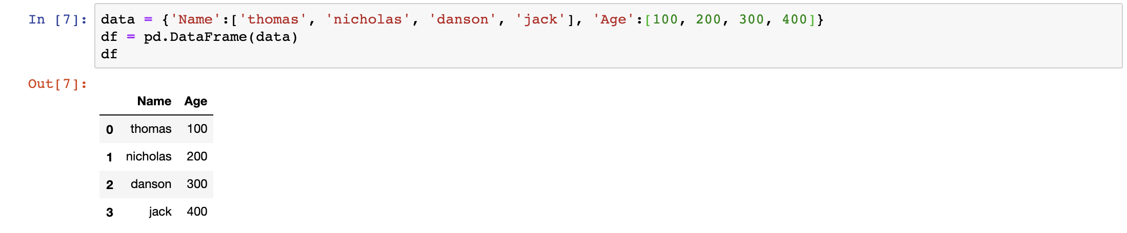
dictionary

data = {‘Name’:[‘thomas’, ‘nicholas’, ‘danson’, ‘jack’], ‘Age’:[100, 200, 300, 400]} 
df = pd.DataFrame(data)

Usually, we don’t create our own dataframes. Instead, we read explore, manipulate and visualise data in Pandas by importing data to a dataframe.
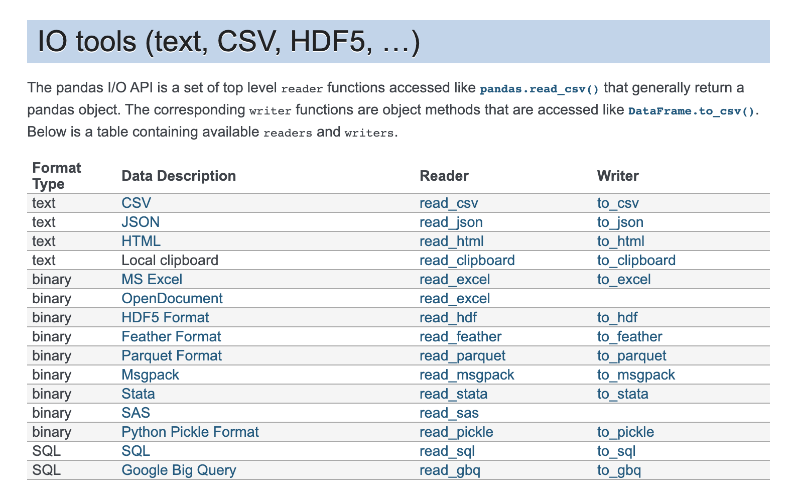
Pandas can read from multiple formats, but the usual one is csv.
Here’s the official list of file types pandas can read from.

We will import the Titanic Dataset here.

df = pd.read_csv(filepath)

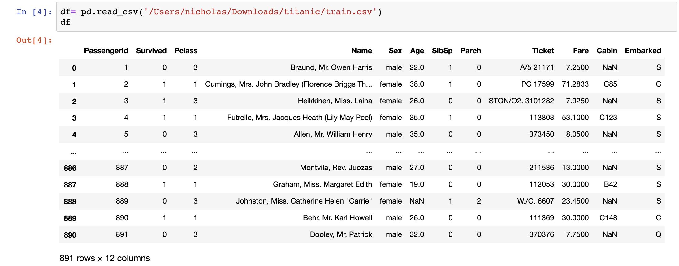
The main objective of this dataset is to study what are the factors that affect the survivability of a person onboard the titanic. Let’s explore the data to find out exactly that.

After importing your data, you want to get a feel for it.
Here are some basic operations:

Summary of the dataset

df.info()

By this command alone we can already tell the number of rows and columns, data types of the columns and if null values exist in them.

Unique Values for each column

df.unique()

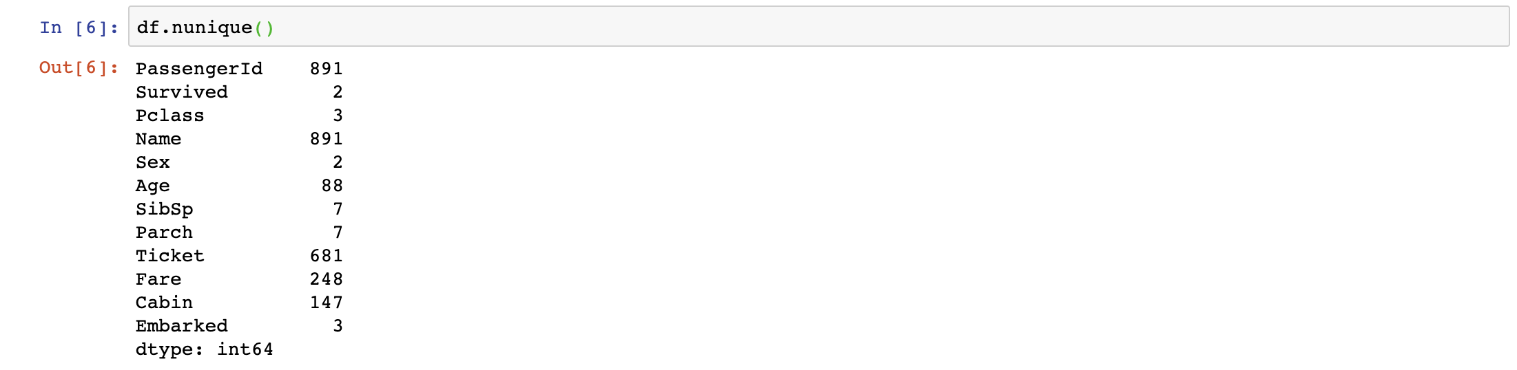
The df.unique() command allows us to better understand what does each column mean. Looking at the Survived and Sex columns, they only have 2 unique values. It usually means that they are categorical columns, in this case, it should be True or False for Survived and Male or Female for Sex.

We can also observe other categorical columns like Embarked, Pclass and more. We can’t really tell what does Pclass stand for, let’s explore more.

Selection of Data

It is extremely easy to select the data you want in Pandas.
Let’s say we want to only look at the Pclass column now.

df[‘Pclass’]

We observe that the 3 unique values are literally 1,2 and 3 which stands for 1st class, 2nd class and 3rd class. We understand that now.

We can also select multiple columns at once.

df[[‘Pclass’,’Sex’]]

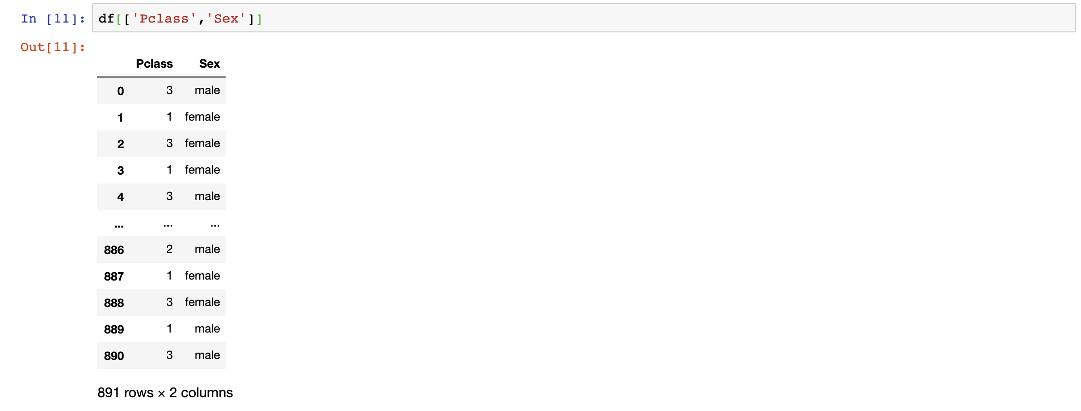
This command is extremely useful for including/excluding columns you need/don’t need.

Since we don’t need the name, passenger_id and ticket because they play no role at all in deciding if the passenger survives or not, we are excluding these columns in the dataset and it can be done in 2 ways.

df= df[[‘Survived’,’Pclass’,’Sex’,’Age’,’SibSp’,’Parch’,’Fare’,’Cabin’,’Embarked’]]ordf.drop(['PassengerId', 'Name', 'Ticket'], axis = 1, inplace=True)

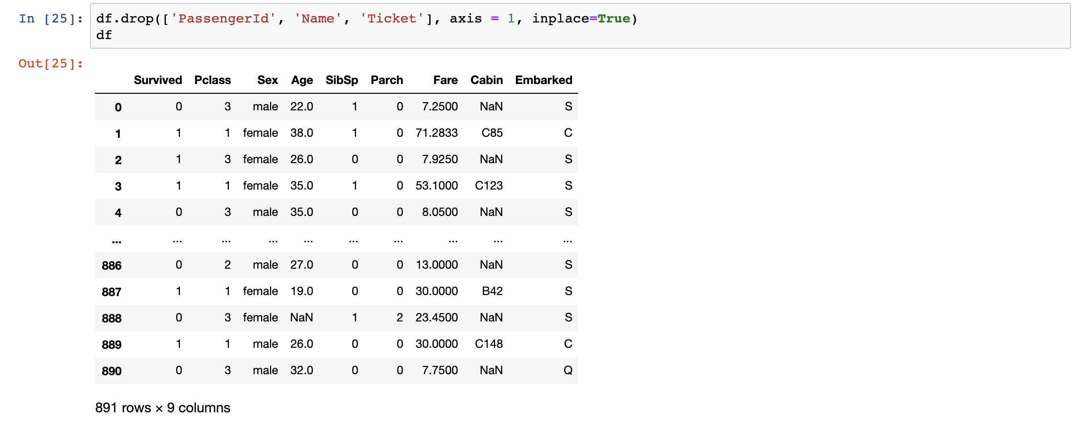
The inplace=True parameter tells Pandas to auto assign what you intend to do to the original variable itself, in this case it is df.

We can also select data by rows. Let’s say that we want to investigate the 300th to 310th rows of the dataset.

df.iloc[500:511]

It works just like a python list, where the first number(500) of the interval is inclusive and the last number(511) of the interval is exclusive.

Conditional Selection

We can also filter through the data. Let’s say we want to only observe the data for male passengers.

df[df['Sex'] == 'male']

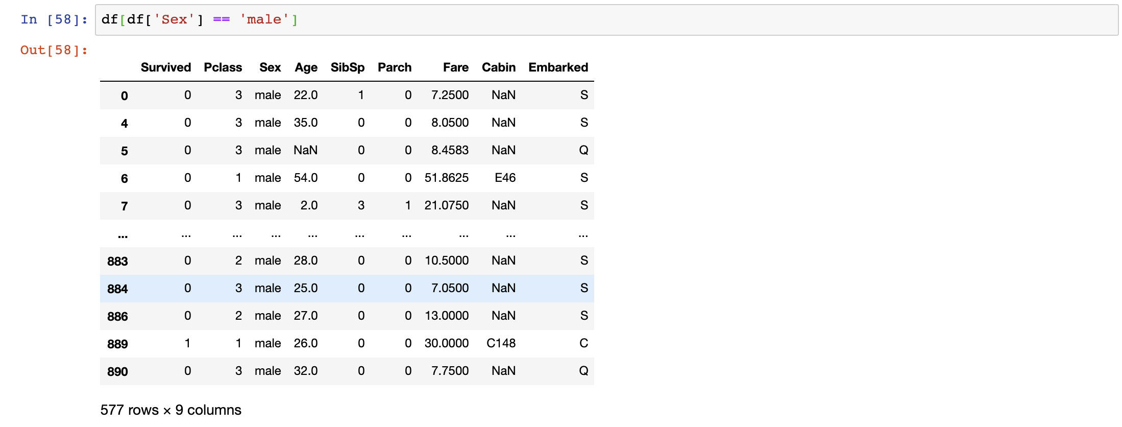
The command df[‘Sex’] == ‘male’ will return a Boolean for each row. Nesting a df[] over it will return the whole dataset for male passengers.
That’s how Pandas work.

This command is extremely powerful for visualising data in the future.
Let’s combine what we had learnt so far.

df[[‘Pclass’,’Sex’]][df[‘Sex’] == ‘male’].iloc[500:511]

With this command, we are displaying only 500th to 510th row of the Pclass and Sex Column for Male Passengers. Play around with the commands to get comfortable using them.

Aggregation Functions

Now that we know how to navigate through data, it is time to do some aggregation upon it. To start off, we can use the describe function to find out the distribution, max, minimum and useful statistics of our dataset.

df.describe()

Note that only numerical columns will be included in these mathematical commands. Other columns will be automatically excluded.

We can also run the following commands to return the respective aggregations, note that the aggregations can be run by conditional selection as well.

df.max()
df[‘Pclass’].min()
df.iloc[100:151].mean()
df.median()
df.count()
df.std()

We can also do a correlation matrix against the columns to find out their relationship with each other.

df.corr()

It looks like top 3 numerical columns that are contributing to the survivability of the passengers are Fare, Pclass and Parch because they hold the highest absolute values against the survived column.

We can also check the distribution of each column. In a table format, it is easier to interpret distributions for categorical columns.

df[‘Sex’].value_counts()

Looks like our passengers are male dominant.

Data Cleaning

If you’ve kept up, you’ve got a pretty good feel of our data right now.
You want to do some sort of aggregation/visualisation to represent your findings. Before that, you often have to clean up your dataset before you can do anything.

Your dataset can often include dirty data like:

null values
empty values
incorrect timestamp
many many more

We could have already tell if there’s any null values when we used the command df.info(). Here’s another one:

df.isnull().sum()

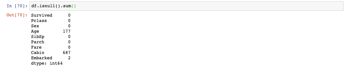
We can see that there are null values in the Age, Cabin and Embarked columns. You can see what the rows look like when the values are null in those specific columns.

df[df[‘Age’].isnull()]

For some reason, all the other data except for Age and Cabin are present here.
It totally depends on you to deal with null values. For simplicity’s sake, we will remove all rows with null values in them.

df.dropna(inplace=True)or#df.dropna(axis=1, inplace=True) to drop columns with null values

We could’ve also replaced all our null values with a value if we wanted to.

df[‘Age’].fillna(df[‘Age’].mean())

This command replaces all the null values in the Age column with the mean value of the Age column. In some cases, this is a good way to handle null values as it doesn’t mess with the skewness of the values.

GroupBy

So now your data is clean. We can start exploring the data through groups. Let’s say we want to find out the average/max/min
(insert numerical column here) for a passenger in each Pclass.

df.groupby(‘Pclass’).mean()
or
df.groupby('Pclass')['Age'].mean()

This tells us many things. For starters, it tells us the average ages and fares for each Pclass. It looks like the 1st class has the most expensive fares, and they are the oldest among the classes. Makes sense.

We can also layer the groups. Let’s say now we also want to know for each Pclass, the average ages and fares for males and females.

df.groupby([‘Pclass’,’Sex’]).mean()

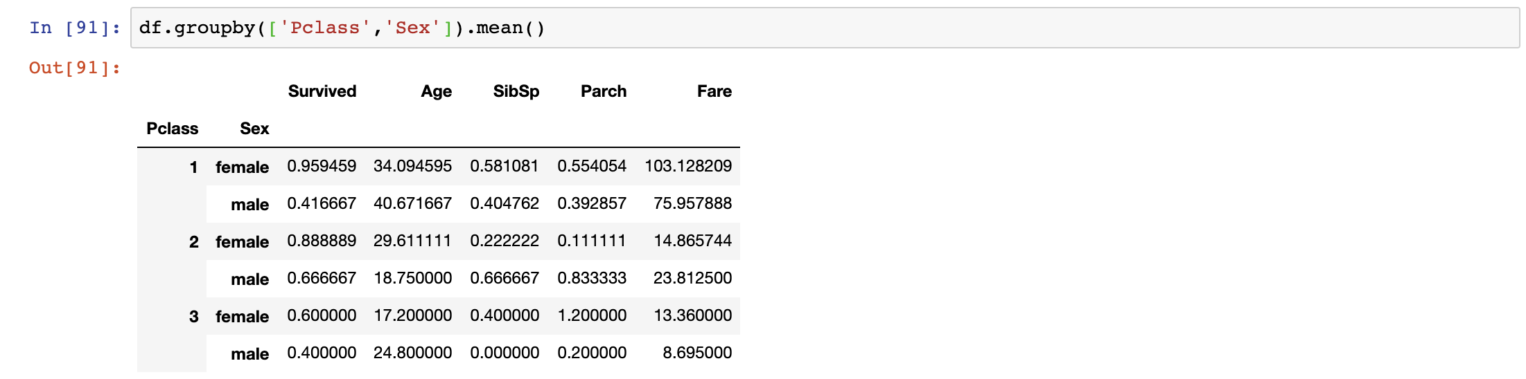
We do that by simply passing the list of groups through the GroupBy Function. We can start to analyse and make certain hypothesis based on these complex GroupBy. One observation I can make is that the Average Fare for Females in 1st Class is the highest among all the passengers, and they have the highest survivability as well. On the flip side, the Average Fare for Males in
3rd Class is the lowest and has the lowest survivability.

I guess money do save lives.

Concatenation and Merging

After some analysis, we figured that we need to add some row/columns to our data. We can easily do that with concatenation and merging dataframes.
We add rows by:

first_5 = df.head()
last_5 = df[178:]
combined = pd.concat([first_5,last_5], axis = 0)

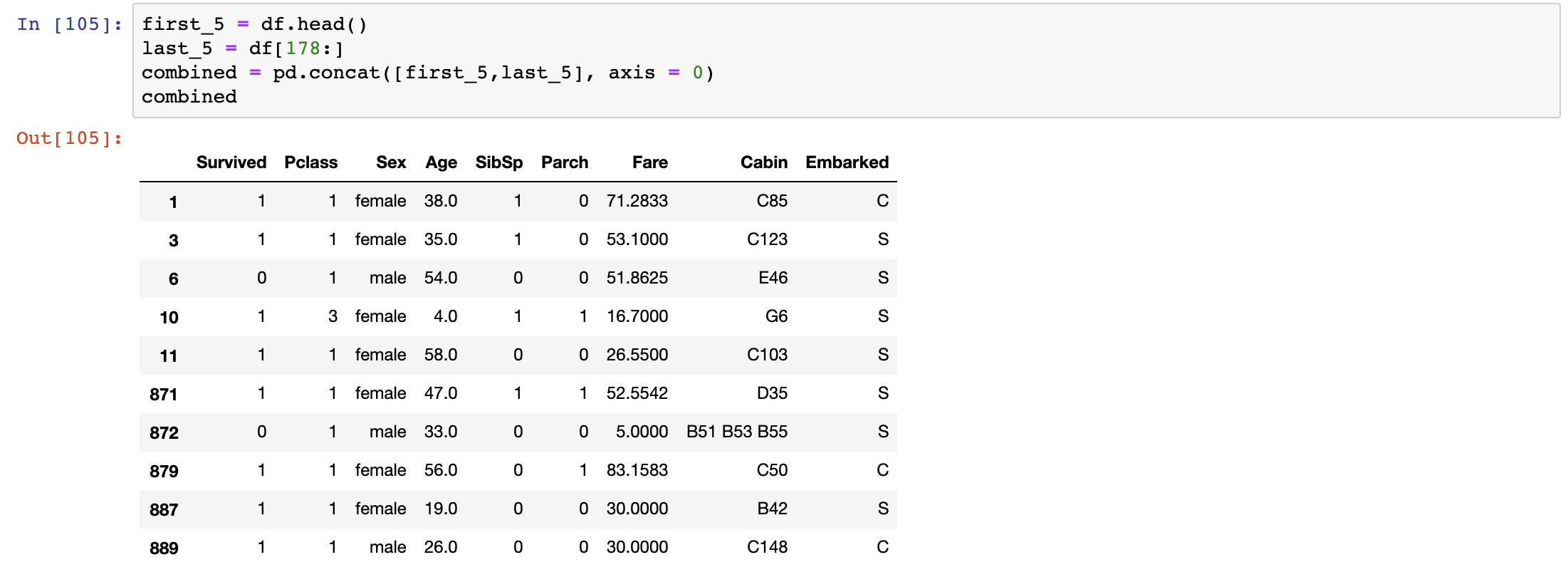
Note that when you concatenate, the columns have to match between dataframes. It works just like a SQL Union.

Now what if we want to add columns by joining.
We merge.

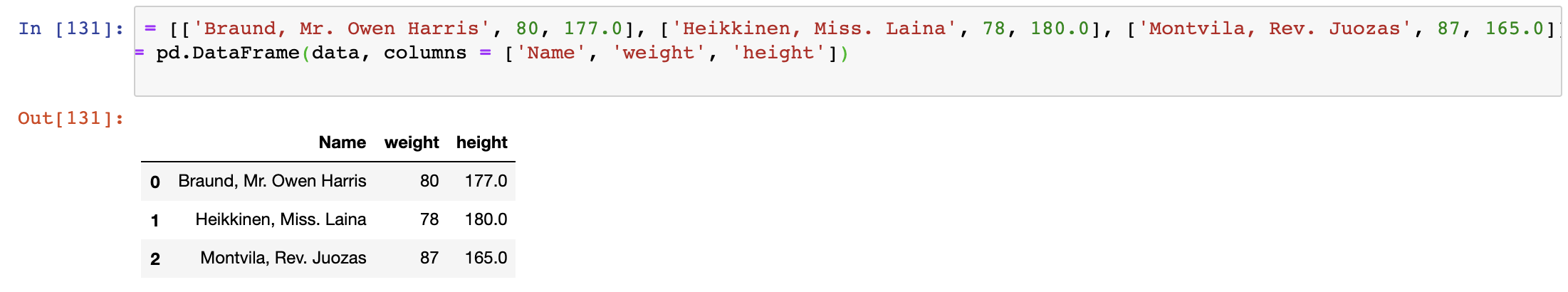
Say we had an external dataset that contained the weight and height of the passengers onboard. For this, I’m going to create my own dataset for 3 passengers.

data = [[‘Braund, Mr. Owen Harris’, 80, 177.0], [‘Heikkinen, Miss. Laina’, 78, 180.0], [‘Montvila, Rev. Juozas’, 87, 165.0]] 
df2 = pd.DataFrame(data, columns = [‘Name’, ‘weight’, ‘height’])

Now we want to add the weight and height data into our titanic dataset.

df3 = pd.merge(df,df2, how=’right’, on=’Name’)

The merge works exactly like SQL joins, with methods of left, right, outer and inner. I used the right join here to display only the passengers who had weight and height recorded. If we had used a left join, the result will show the full titanic dataset with nulls where height and weight are unavailable.

df3 = pd.merge(df,df2, how=’left’, on=’Name’)

Data Manipulation

We now move into more advanced territory where we want to heavily manipulate the values in our data. We may want to add our own custom columns, change the type of values or even implement complex functions into our data.

Data Types

This is a fairly straight forward manipulation. Sometimes we may want to change the type of data to open possibilities to other functions. A very good example is changing ‘4,000’ which is a str into an int ‘4000’.

Let’s change our weight data which is in float right now to integer.

df2[‘weight’].astype(int)

Note that the astype() function goes through every row of the data and tries to change the type of data into whatever you mentioned. Hence, there are certain rules to follow for each type of data.

For example:

data can’t be null or empty
when changing float to integer, the decimals have to be in .0 form

Hence, the astype() function can be tricky at times.

Apply Function

The apply function is one of the most powerful functions in pandas.
It lets you manipulate the data in whatever form you want to. Here’s how.

Step 1: Define a functionAssume we want to rename the Pclass to their actual names.
1 = 1st Class
2 = 2nd Class
3 = 3rd Class

We first define a function.

def pclass_name(x):
    if x == 1:
        x = '1st Class'
    if x == 2:
        x = '2nd Class'
    if x == 3:
        x = '3rd Class'
    return x

Step 2: Apply the functionWe can then apply the function to each of the values of Pclass column.
The process will pass every record of the Pclass column through the function.

df3[‘Pclass’] = df3[‘Pclass’].apply(lambda x: pclass_name(x))

The records for Pclass columns has now changed.
It really is up to your imagination on how you want to manipulate your data.
Here’s where you can be creative.

Custom Columns

Sometimes, we want to create custom columns to allow us to better interpret our data. For example, let’s create a column with the BMI of the passengers.

The formula for BMI is:

weight(kg) / height²(m)

Hence, let’s first convert our height values which is in cm to m and square the values. We shall use the apply function we had just learnt to achieve that.

def convert_to_bmi(x):
 x = (x/100)**2
 return xdf4[‘height’] = df4[‘height’].apply(lambda x: convert_to_bmi(x))

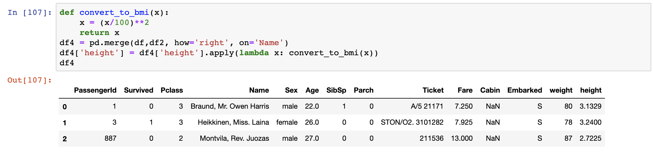
We then create a new column where the values are weight divided by height.

df4[‘BMI’] = df4[‘weight’]/df4[‘height’]

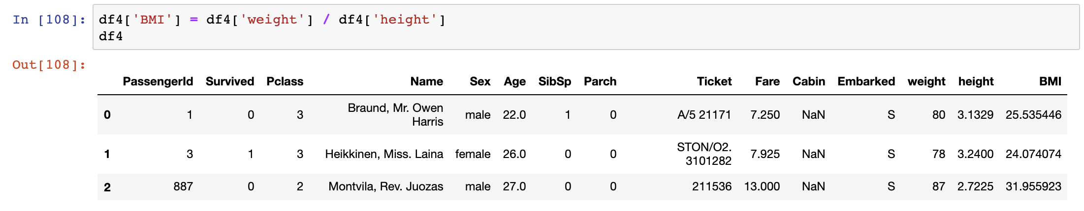
If we had all the BMIs for the passengers, we can then make further conclusions with the BMI, but I’m not going into that. You get the point.

Finalising and Export

After everything’s done, you may want to sort and rename the columns.

df3.rename(columns={'BMI':'Body_Mass_Index','PassengerId':'PassengerNo'}, inplace = True)df3 = df3.sort_values('Body_Mass_Index')

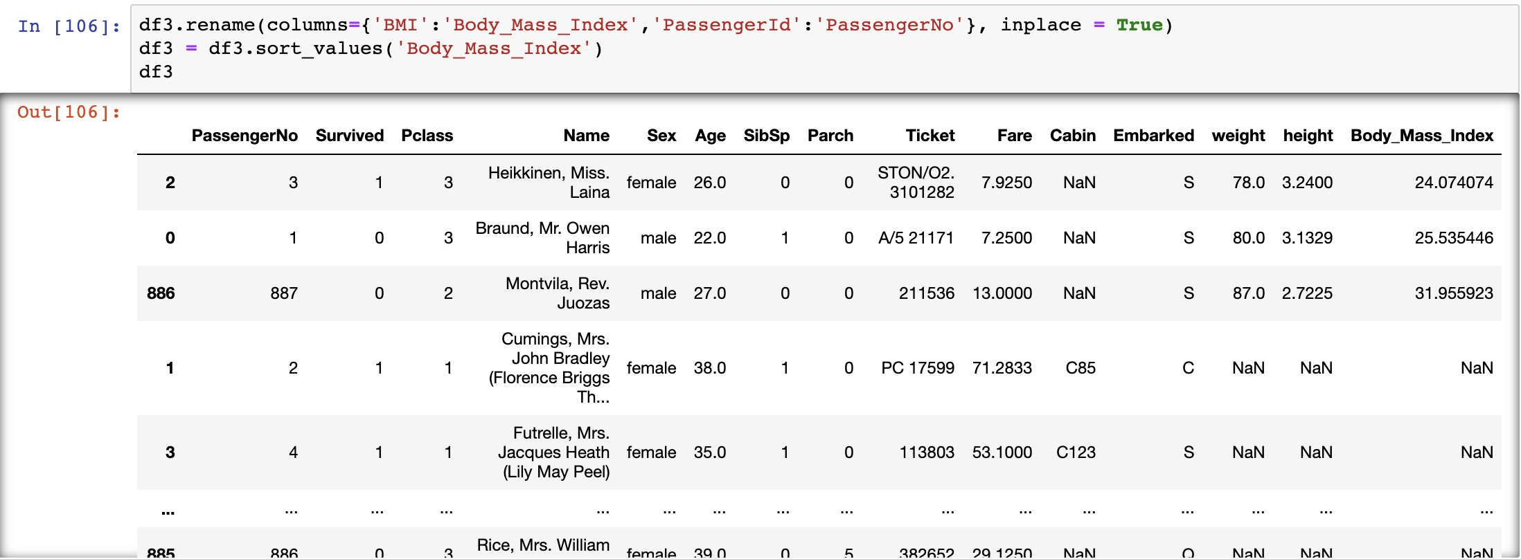
We had renamed the BMI to its full name and sort rows by BMI here.
Note that after sorting, the index do not change so that information is not lost.

Last but not least,
we can export our data into multiple formats (refer to list on top).
Let's export our data as a csv file.

df3.to_csv(filepath)

Conclusion

Give yourself a pat on the back if you’ve made it this far.
You have officially mastered the basics of Pandas,
a necessary tool for every data scientist.

What you had learnt today:

Creating and Importing Dataframes
Summary Functions of Dataframes
Navigating through Dataframes
Aggregation of Values
Cleaning Up Data
GroupBy
Concatenation and Merging
Data Manipulation (*** apply function ***)
Finalising and Exporting

Keep it scarred in your brain as I swear you will use it often in the future.
As always, I end with a quote.

You can have data without information,
but you can’t have information without data — Daniel Keys Moran

Thanks for reading! If you want to get in touch with me, feel free to reach me on nickmydata@gmail.com or my linkedIn Profile. You can also view the code in my Github.

Search This Blog

Subrat's Technical Blog