Building a machine learning classifier model for diabetes
Based on medical diagnostic measurements
Python codes are available: https://github.com/JNYH/diabetes_classifier
The Pima Indians of Arizona and Mexico have the highest reported prevalence of diabetes of any population in the world. A small study has been conducted to analyse their medical records to assess if it is possible to predict the onset of diabetes based on diagnostic measures.


The dataset is downloaded from Kaggle, where all patients included are females at least 21 years old of Pima Indian heritage.
The objective of this project is to build a predictive machine learning model to predict based on diagnostic measurements whether a patient has diabetes.


This is a binary (2-class) classification project with supervised learning. A Jupyter Notebook with Python codes is available for download on my GitHub, so you can follow the process below.
Step 1: Import relevant libraries
Standard libraries of Pandas and Numpy are imported, along with visualisation libraries of Matplotlib and Seaborn. There are also a host of models and measurement metrics imported from Scikit-Learn library.
Step 2: Read in data, perform Exploratory Data Analysis (EDA)
Use Pandas to read the csv file “diabetes.csv”. There are 768 observations with 8 medical predictor features (input) and 1 target variable (output 0 for ”no” or 1 for ”yes”). Let’s check the target variable distribution:
df = pd.read_csv('diabetes.csv')
print(df.Outcome.value_counts())
df['Outcome'].value_counts().plot('bar').set_title('Diabetes Outcome')


This two-class dataset seems imbalanced. As a result, there is a possibility that one class is over-represented and the model built might be biased towards to majority. I have tried to solve this by oversample the smaller class but there was no improvement. See Appendix at the end of the notebook.
The 8 medical predictor features are:
· Pregnancies: Number of times pregnant
· Glucose: Plasma glucose concentration a 2 hours in an oral glucose tolerance test
· BloodPressure: Diastolic blood pressure (mm Hg)
· SkinThickness: Triceps skin fold thickness (mm)
· Insulin: 2-Hour serum insulin (mu U/ml)
· BMI: Body mass index (weight in kg/(height in m)²)
· DiabetesPedigreeFunction: Diabetes pedigree function
· Age: Age (years)
features = ['Pregnancies', 'Glucose', 'BloodPressure', 'SkinThickness', 'Insulin', 'BMI', 'DiabetesPedigreeFunction', 'Age']ROWS, COLS = 2, 4
fig, ax = plt.subplots(ROWS, COLS, figsize=(18,8) )
row, col = 0, 0
for i, feature in enumerate(features):
    if col == COLS - 1:
        row += 1
    col = i % COLS

    df[feature].hist(bins=35, color='green', alpha=0.5, ax=ax[row, col]).set_title(feature)
The above code is to visualise the distribution of these 8 features.

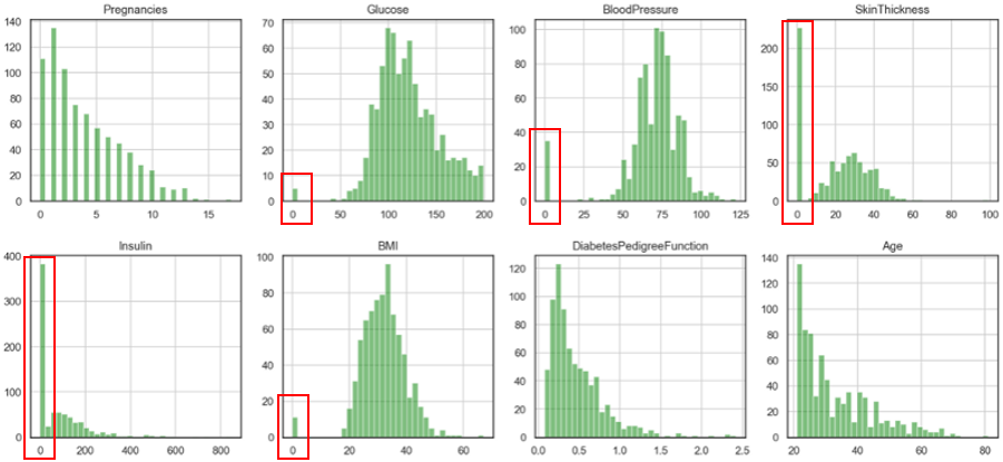
There are some zeros in the data set, which will affect the training accuracy. I have chosen to replace them with the median value.

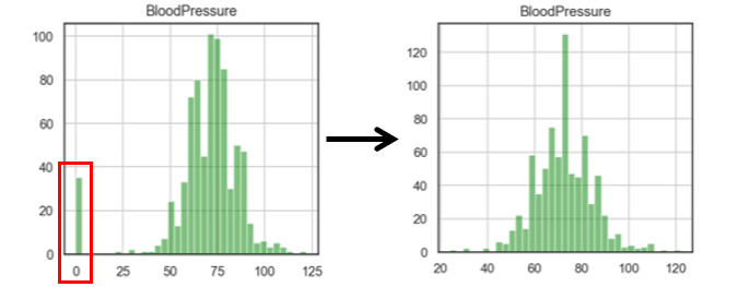
Replacing zeros with median is a two-step process: first replace zero by NaN, then replace NaN by median (because NaN will not influence the median)
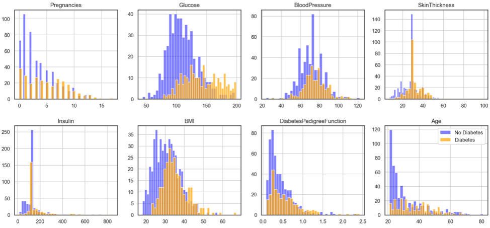
After that we can modify the code to visualise the relative positions of the 2 classes.

Step 3: Create feature (X) and target (y) dataset
The notations X and y are commonly used in Scikit-Learn. I have also used Random Forest Classifier to check feature importance. ‘Glucose’ and ‘BMI’ are the most important medical predictor features.
X, y = df.drop('Outcome', axis=1), df['Outcome']rfc = RandomForestClassifier(random_state=SEED, n_estimators=100)rfc_model = rfc.fit(X, y)(pd.Series(rfc_model.feature_importances_, index=X.columns)
    .nlargest(8)
    .plot(kind='barh', figsize=[8,4])
    .invert_yaxis())plt.yticks(size=15)
plt.title('Top Features derived by Random Forest', size=20)


Step 4: Split data to 80:20 ratio, and perform Model Selection
The standard code to split data for training and testing:
from sklearn.model_selection import train_test_split
X_train, X_test, y_train, y_test = train_test_split(X, y, test_size=.2, random_state=SEED)
After that is a bunch of code do a baseline model evaluation, while I explain the purpose of below 2 lines of code:
model.fit(X_train, y_train) — using the training input data and target value to teach the model. After this command, the model will learn the ‘rules’ and ’knowledge’ of differentiating an onset diabetes and non-diabetes patient.
y_pred = model.predict(X_test) — the trained model is then used to make predictions using X_test as inputs, and the predicted results are stored in y_pred. After that we can compare y_test (the reality) with y_pred (model prediction). If the model has learnt all the ‘knowledge’, y_pred will be 100% match with y_test.
Below 9 models have been evaluated:
· Gaussian Naive Bayes
· Bernoulli Naive Bayes
· Multinomial Naive Bayes
· Logistic Regression
· K Nearest Neighbour
· Decision Tree Classifier
· Random Forest Classifier
· Support Vector Classification (SVC)
· Linear SVC
· Gaussian Naive Bayes
· Bernoulli Naive Bayes
· Multinomial Naive Bayes
· Logistic Regression
· K Nearest Neighbour
· Decision Tree Classifier
· Random Forest Classifier
· Support Vector Classification (SVC)
· Linear SVC
The performance metrics used in the evaluation are:
· Accuracy Score: proportion of correct predictions out of the whole dataset. Be careful when the target class is imbalance, for example, if a useless model predicts all flight passengers as non-terrorist, then the model would be 99.99% accurate.
· Precision Score: proportion of correct predictions out of all predicted diabetic cases.
· Recall Score: proportion of correct predictions out of all true diabetic cases.
· F1 Score: optimised balance between Precision and Recall for binary targets.
· Area Under ROC Curve: prediction scores from area under Receiver Operating Characteristic (ROC) curve, which is a relationship between True Positive Rate and False Positive Rate.
· Log Loss: aka logistic loss or cross-entropy loss, defined as the negative log-likelihood of the true labels given a probabilistic classifier’s predictions, and has to be as low as possible.
Evaluation results:

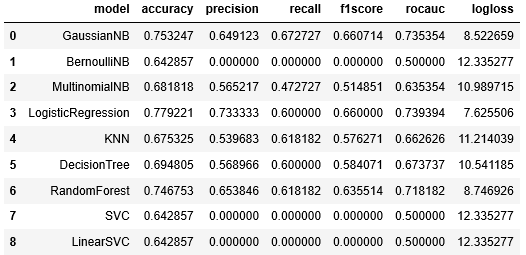
From the above metric scores, these 3 models seem to be leading: GaussianNB, LogisticRegression, and RandomForest.
Step 5: Optimise model: hyperparameter tuning
In the usual data science methodology, I should proceed to tune the hyperparameters of the 3 leading models. But for learning sake, I have added a bunch of codes to tune ALL models, especially their threshold.
For the metric “Area Under ROC Curve”, Logistic Regression seems to have fallen behind a little, leaving 2 leading models to choose from.


F1-Score has improved for all models after tuning the threshold and other hyperparameters.


It seems like a neck-to-neck race, and we need a tie breaker. Below metrics are Log-Loss and Time Taken, where scores should be as low as possible.

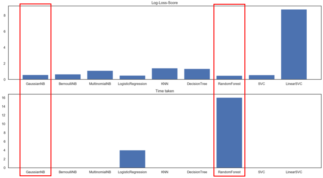
Random Forest is too time consuming to run, and thus Gaussian Naive Bayes is the winning model! Here are the performance metric scores after tuning:


It is laborious to compare these new scores with the previous table (baseline model performance). So I wrote a for-loop to compare every cell, indicating 1 when the metric has improved, and 0 when there is no improvement.


Final results
The relevance of diabetes classification is NOT to misclassify a diabetic patient as normal, so the focus should be on “Recall” metric. Gaussian Naive Bayes has scored the highest for both Recall Score as well as F1-Score.


Conclusion
In this project, the Gaussian Naive Bayes model has achieved prediction score of 90.9%, ie, out of all diabetic patients, 90.9% of them will be correctly classified using medical diagnostic measurements.
‘Glucose’ and ‘BMI’ are the most important medical predictor features.
For a healthy living, look after your sugar intake and your weight.
I wish all a healthy life!
Python codes for the above analysis are available on my GitHub, do feel free to refer to them.


2 comments:
The information provided is really great and would love to share it with others.
must also visit
Diabetes mellitus
Very Informative and creative contents. This concept is a good way to enhance the knowledge. thanks for sharing. Continue to share your knowledge through articles like these, and keep posting on
Data Engineering Services
Artificial Intelligence Solutions
Post a Comment