Background
This article is the fourth in the series on the time-series data. We started by discussing various exploratory analyses along with data preparation techniques followed by building a robust model evaluation framework. And finally, in our previous article, we discussed a wide range of classical forecasting techniques that must be explored before moving to machine learning algorithms.
Now, in the current article, we are going to apply all these learnings to a real-life dataset. We will work through a time series forecasting project from end-to-end, from importing the dataset, analyzing and transforming the time series to training the model, and making predictions on new data. The steps of this project that we will work through are as follows:
- Problem Description
- Data Preparation and Analysis
- Set up an Evaluation Framework
- Stationary Check: Augmented Dickey-Fuller test
- ARIMA Models
- Residual Analysis
- Bias corrected Model
- Model Validation
Problem Description
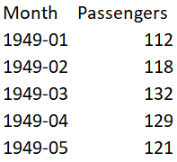
The problem is to predict the number of monthly airline passengers. We will use the Airline Passengers dataset for this exercise. This dataset describes the total number of airline passengers over time. The units are a count of the number of airline passengers in thousands. There are 144 monthly observations from 1949 to 1960. Below is a sample of the first few rows of the dataset.

You can download this dataset from here.
Python Libraries for this Project
We need the following libraries to work on this project. These names are self-explanatory but don’t worry if you are not getting any of them. As we go along you will understand the usage of these libraries.
import numpy
from pandas import read_csv
from sklearn.metrics import mean_squared_error
from math import sqrt
from math import log
from math import exp
from scipy.stats import boxcox
from pandas import DataFrame
from pandas import Grouper
from pandas import Series
from pandas import concat
from pandas.plotting import lag_plot
from matplotlib import pyplot
from statsmodels.tsa.stattools import adfuller
from statsmodels.tsa.arima_model import ARIMA
from statsmodels.tsa.arima_model import ARIMAResults
from statsmodels.tsa.seasonal import seasonal_decompose
from statsmodels.graphics.tsaplots import plot_acf
from statsmodels.graphics.tsaplots import plot_pacf
from statsmodels.graphics.gofplots import qqplot
Data Preparation and Analysis
We will use the read_csv() function to load the time series data as a series object, a one-dimensional array with a time label for each row. It is always good to take a peek at the data to confirm that data has been loaded correctly.
series = read_csv('airline-passengers.csv', header=0, index_col=0, parse_dates=True, squeeze=True)
print(series.head())

Let’s begin the data analysis by looking into the summary statistics, we will get a quick idea of the data distribution.
print(series.describe())

We can see the number of observations matches our expectations, the mean is about 280 which we can consider our level in this series. Other statistics like standard deviation and percentiles suggest a large spread of the data.
As a next step, we will visualize the values on a line plot, this tool can provide a lot of insights into the problem.
series.plot()
pyplot.show()

Here, the line plot suggests that there is an increasing trend of airline passengers over time. We can also observe a systematic seasonality to the travel pattern for each year and the seasonal signal appears to be growing over time, which suggests a multiplicative relationship.
This insight gives us a hint that data may not be stationary and we can explore differencing with one or two levels to make it stationary before modeling.
We can confirm our assumption by yearly line plots.
For the following plot, created year-wise separate groups of data and plotted a line plot for each year from 1949 to 1957. You can create this plot for any number of years.
groups = series['1949':'1957'].groupby(Grouper(freq='A'))
years = DataFrame()
pyplot.figure()
i = 1
n_groups = len(groups)
for name, group in groups:
  pyplot.subplot((n_groups*100) + 10 + i)
  i += 1
  pyplot.plot(group)
pyplot.show()

We can observe that seasonality is a yearly cycle by looking at line plots of the dataset by year. We can see a dip at each year-end and rise from July to August. This pattern exists across the years which again suggests us to adopt season based modeling.
Let’s explore the density of observations for further insight into our data structure.
pyplot.figure(1)
pyplot.subplot(211)
series.hist()
pyplot.subplot(212)
series.plot(kind='kde')
pyplot.show()

We can observe that the distribution is not Gaussian, and this insight encourages us to explore some log or power transforms of the data before modeling.
Let’s analyze monthly data by year and get an idea of the spread of observations for each year.
We will perform this analysis through a box and whisker plot.
groups = series['1949':'1960'].groupby(Grouper(freq='A'))
years = DataFrame()
for name, group in groups:
  years[name.year] = group.values
years.boxplot()
pyplot.show()
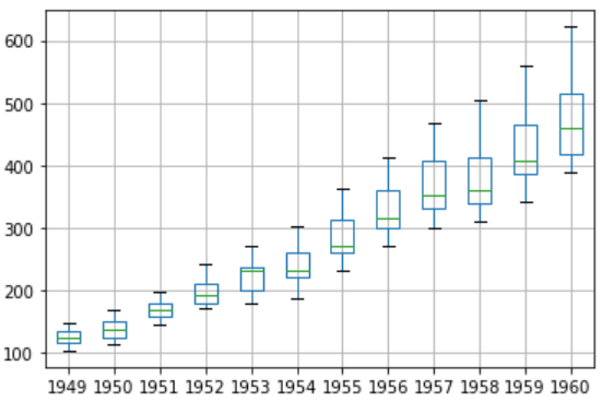
The spread of the data (blue boxes) suggests a growth trend over the years which also suggests our assumption of non-stationarity of the data.
Decompose the time series for more clarity on its components — Level, Trend, Seasonality, and Noise.
Based on our analysis till now, we have an intuition that out time series is multiplicative. So, we can decompose the series assuming a multiplicative model.
result = seasonal_decompose(series, model='multiplicative')
result.plot()
pyplot.show()

We can see that the trend and seasonality information extracted from the series validate our earlier findings that series has a growing trend and yearly seasonality. The residuals are also interesting, showing periods of high variability in the early and later years of the series.
Set up an Evaluation Framework to Build a Robust Model
Before proceeding to model building exercise we must develop an evaluation framework to assess the data and evaluate different models.
The first step is defining a validation dataset
This is historical data, so we cannot collect the updated data from the future to validate this model. Therefore, we will use the last 12 months of the same series as the validation dataset. We will split this time series into two subsets — training and validation, throughout this exercise we will use this training dataset named ‘dataset’ to build and test different models. The selected models will be validated through the ‘validation’ dataset.
series = read_csv('airline-passengers.csv', header=0, index_col=0, parse_dates=True, squeeze=True)
split_point = len(series) - 12
dataset, validation = series[0:split_point], series[split_point:]
print('Train-Dataset: %d, Validation-Dataset: %d' % (len(dataset), len(validation)))
dataset.to_csv('dataset.csv', header=False)
validation.to_csv('validation.csv', header=False)

We can see the training set has 132 observations and the validation set has 12 observations.
The second step is developing a baseline model.
The baseline prediction for time series forecasting is also known as the naive forecast. In this approach value at the previous timestamp is the forecast for the next timestamp.
We will use the walk-forward validation which is also considered as a k-fold cross-validation technique of the time series world. You can explore this technique in detail in one of my previous articles “Build Evaluation Framework for Forecast Models”.
series = read_csv('dataset.csv', header=None, index_col=0, parse_dates=True, squeeze=True)
X = series.values
X = X.astype('float32')
train_size = int(len(X) * 0.5)
train, test = X[0:train_size], X[train_size:]
Here is the implementation of our Naive model and walk forward validation result for single-step forecasts.
history = [x for x in train]
predictions = list()
for i in range(len(test)):
  yhat = history[-1]
  predictions.append(yhat)
  obs = test[i]
  history.append(obs)
  print('>Forecast=%.3f, Actual=%3.f' % (yhat, obs))
# display performance report
rmse = sqrt(mean_squared_error(test, predictions))
print('RMSE: %.3f' % rmse)
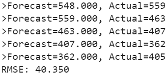
As a performance measure, we have used RMSE (root mean squared error). Now, we have a baseline model accuracy result, RMSE: 40.350
Our goal is to build a model with higher accuracy than this baseline.
Stationary Check — Augmented Dickey-Fuller test
We already have some evidence from insights generated from exploratory data analysis that our time series is non-stationary.
We will confirm our hypothesis using this Augmented Dickey-Fuller test. This is a statistical test, It uses an autoregressive model and optimizes an information criterion across multiple different lag values.
The null hypothesis of the test is that the time series is not stationary.
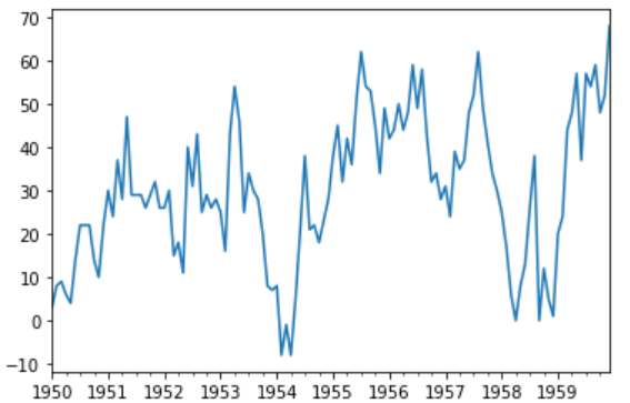
As we have a strong intuition that time series is not stationary, so let’s create a new series with differenced values and check this transformed series for stationarity.
Let’s create a differenced series.
We will subtract the previous year’s same month value from the current value to make this new series.
def difference(dataset, interval=1):
  diff = list()
  for i in range(interval, len(dataset)):
    value = dataset[i] - dataset[i - interval]
    diff.append(value)
  return Series(diff)
X = series.values
X = X.astype('float32')# differenced datamonths_in_year = 12
stationary = difference(X, months_in_year)
stationary.index = series.index[months_in_year:]
Now, we can apply the ADF test on the differenced series as below.
We will use adfuller function to test our hypothesis as below.
result = adfuller(stationary)
print('ADF Statistic: %f' % result[0])
print('p-value: %f' % result[1])
print('Critical Values:')
for key, value in result[4].items():
  print('\t%s: %.3f' % (key, value))

The results show that the test statistic value -3.048011 is smaller than the critical value at 1% of -3.488. This suggests that we can reject the null hypothesis with a significance level of less than 1%.
Rejecting the null hypothesis means that the time series is stationary.
Let’s visualize the differenced dataset.
We can see a pattern in the plot looks random, does not show any trend or seasonality.
stationary.plot()
pyplot.show()
It’s ideal to use a differenced dataset as the input for our ARIMA model. As we know this dataset is stationary, therefore parameter ‘d’ can see set to 0.
Next, we have to decide lag values for Autoregression (AR) and Moving Average (MA) parameters.
These parameters are also known as p and q respectively. we can identify these parameters using Autocorrelation Function (ACF) and Partial Autocorrelation Function (PACF).
pyplot.figure()
pyplot.subplot(211)
plot_acf(stationary, lags=25, ax=pyplot.gca())
pyplot.subplot(212)
plot_pacf(stationary, lags=25, ax=pyplot.gca())
pyplot.show()

ACF shows a significant lag of 4 months, which means an ideal value for p is 4. PACF shows a significant lag of 1 month, which means an ideal value for q is 1.
Now, we have all the required parameters for the ARIMA model.
- Autoregression parameter (p): 4
- Integrated (d): 0 (We could have used 1, had we considered original observations as the input. We have seen our series transformed into stationary after one level of differencing)
- Moving Average parameter (q): 1
Let’s create a function to invert differenced value
As we are modeling on a differenced dataset, we have to bring back the predicted values at the original scale by adding the same month value from the previous year.
def inverse_difference(history, yhat, interval=1):
  return yhat + history[-interval]
ARIMA model using manually identified parameters
history = [x for x in train]
predictions = list()
for i in range(len(test)):
  # difference data
  months_in_year = 12
  diff = difference(history, months_in_year)
  # predict
  model = ARIMA(diff, order=(3,0,1))
  model_fit = model.fit(trend='nc', disp=0)
  yhat = model_fit.forecast()[0]
  yhat = inverse_difference(history, yhat, months_in_year)
  predictions.append(yhat)
  # observation
  obs = test[i]
  history.append(obs)
  print('>Forecast=%.3f, Actual=%.3f' % (yhat, obs))
# report performance
rmse = sqrt(mean_squared_error(test, predictions))
print('RMSE: %.3f' % rmse)

We can see, an error has reduced significantly as compared to baseline.
We will further try to optimize the parameters using Grid Search
We will evaluate multiple ARIMA models with varying parameter (p,d,q) values.
# grid search ARIMA parameters for time series
# evaluate an ARIMA model for a given order (p,d,q) and return RMSE
def evaluate_arima_model(X, arima_order):
  # prepare training dataset
  X = X.astype('float32')
  train_size = int(len(X) * 0.66)
  train, test = X[0:train_size], X[train_size:]
  history = [x for x in train]
  # make predictions
  predictions = list()
  for t in range(len(test)):
    # difference data
    months_in_year = 12
    diff = difference(history, months_in_year)
    model = ARIMA(diff, order=arima_order)
    model_fit = model.fit(trend='nc', disp=0)
    yhat = model_fit.forecast()[0]
    yhat = inverse_difference(history, yhat, months_in_year)
    predictions.append(yhat)
    history.append(test[t])
  # calculate out of sample error
  rmse = sqrt(mean_squared_error(test, predictions))
  return rmse
# evaluate combinations of p, d and q values for an ARIMA model
def evaluate_models(dataset, p_values, d_values, q_values):
  dataset = dataset.astype('float32')
  best_score, best_cfg = float("inf"), None
  for p in p_values:
    for d in d_values:
      for q in q_values:
        order = (p,d,q)
        try:
          rmse = evaluate_arima_model(dataset, order)
          if rmse < best_score:
            best_score, best_param = rmse, order
          print('ARIMA%s RMSE=%.3f' % (order,rmse))
        except:
          continue
print('Best ARIMA%s RMSE=%.3f' % (best_param, best_score))
# load dataset
series = read_csv('dataset.csv', header=None, index_col=0, parse_dates=True, squeeze=True)
# evaluate parameters
p_values = range(0, 5)
d_values = range(0, 2)
q_values = range(0, 2)
warnings.filterwarnings("ignore")
evaluate_models(series.values, p_values, d_values, q_values)

We have found the best parameters through the grid search. We can further reduce the errors by using suggested parameters (1,1,1).
RMSE: 10.845
Residual Analysis
A final check is to analyze residual errors of the model. Ideally, the distribution of the residuals should follow a Gaussian distribution with a zero mean. We can calculate residuals by substracting predicted values from actuals as below.
residuals = [test[i]-predictions[i] for i in range(len(test))]
residuals = DataFrame(residuals)
print(residuals.describe())
And then simply use describe function to get summary statistics.


We can see, there is a very small bias in the model. Ideally, the mean should have been zero. We will use this mean value (0.810541) to correct the bias in our prediction by adding this value to each forecast.
Bias Corrected Model
As a last improvement to the model, we will produce a biased adjusted forecast. Here is the Python implementation.
history = [x for x in train]
predictions = list()
bias = 0.810541
for i in range(len(test)):
  # difference data
  months_in_year = 12
  diff = difference(history, months_in_year)
  # predict
  model = ARIMA(diff, order=(1,1,1))
  model_fit = model.fit(trend='nc', disp=0)
  yhat = model_fit.forecast()[0]
  yhat = bias + inverse_difference(history, yhat, months_in_year)
  predictions.append(yhat)
  # observation
  obs = test[i]
  history.append(obs)
# report performance
rmse = sqrt(mean_squared_error(test, predictions))
print('RMSE: %.3f' % rmse)
# errors
residuals = [test[i]-predictions[i] for i in range(len(test))]
residuals = DataFrame(residuals)
print(residuals.describe())

We can see errors have slightly reduced and mean has also shifted towards zero. The graphs also suggest a gaussian distribution.


In our example we had a very small bias, so this bias correction may not have proved to be a significant improvement, but in real-life scenarios, this is an important technique to be explored at the end in case any bias exists.
Check autocorrelation in the residuals
As a final check, we should investigate if there any autocorrelation exists in the residual. If exists, it means there is an opportunity for improvement in the model. Ideally, there should not be any autocorrelation left in the residuals if the model is fitted well.


The graphs suggest that all the autocorrelation has been captured in the model and there is no autocorrelation exists in the residuals.
So, our model has passed all the criteria. We can save this model for later use.
Model Validation
We have finalized the model, now it can be saved as a .pkl file for later use. Bias number can also be saved separately.
model.pkl: This includes the coefficients and all other internal data required for prediction.
model bias.npy: This is the bias value stored in a NumPy array.
bias = 0.810541
# save model
model_fit.save('model.pkl')
numpy.save('model_bias.npy', [bias])
Load the Model and Evaluate on Validation Dataset
This is the final step of this exercise. We will load our saved model along with a bias number and make predictions on the validation dataset.
# load and evaluate the finalized model on the validation dataset
validation = read_csv('validation.csv', header=None, index_col=0, parse_dates=True,squeeze=True)
y = validation.values.astype('float32')
# load model
model_fit = ARIMAResults.load('model.pkl')
bias = numpy.load('model_bias.npy')
# make first prediction
predictions = list()
yhat = float(model_fit.forecast()[0])
yhat = bias + inverse_difference(history, yhat, months_in_year) predictions.append(yhat)
history.append(y[0])
print('>Forecast=%.3f, Actual=%.3f' % (yhat, y[0]))
# rolling forecasts
for i in range(1, len(y)):
# difference data
months_in_year = 12
diff = difference(history, months_in_year)
# predict
model = ARIMA(diff, order=(1,1,0))
model_fit = model.fit(trend='nc', disp=0)
yhat = model_fit.forecast()[0]
yhat = bias + inverse_difference(history, yhat, months_in_year)
predictions.append(yhat)
# observation
obs = y[i]
history.append(obs)
print('>Forecast=%.3f, Actual=%.3f' % (yhat, obs))
# report performance
rmse = sqrt(mean_squared_error(y, predictions))
print('RMSE: %.3f' % rmse)
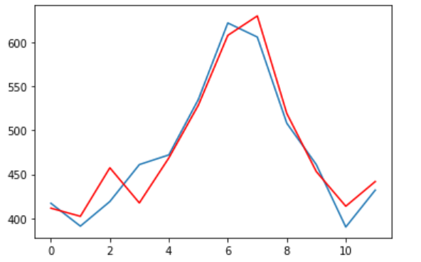
pyplot.plot(y)
pyplot.plot(predictions, color='red')
pyplot.show()We can observe the actual and forecasted values for the validation dataset. These values are also plotted on a line plot which shows a promising result of our model.


You can find the entire code at my Gist repository.
Summary
This tutorial can be used as a template for your univariate time series specific problems. Here, we learned every step involved in any forecasting project, starting from exploratory data analysis to model building, validation, and finally, saving the model for later use.
There are some additional steps that you should explore to improve the result. You can try box cox transformation on the original series and use that as input for the model, apply grid search on the transformed dataset to find optimal parameters.
Thanks for reading! Please feel free to share any comments or feedback.
Hope you found this article informative. In the next few articles, I will discuss some advanced forecasting techniques.


No comments:
Post a Comment