Tips and tricks to create network architecture, train, validate, and save the model and use it to make inferences.
Why Keras, not Tensorflow?
If you are asking, “Should I use keras OR tensorflow?”, you are asking the wrong question.
When I first started my deep-learning journey, I kept thinking these two are completely separate entities. Well, as of mid-2017, they are not! Keras, a neural network API, is now fully integrated within TensorFlow. What does that mean?
It means you have a choice between using the high-level Keras API, or the low-level TensorFlow API. High-level APIs provide more functionality within a single command and are easier to use (in comparison with low-level APIs), which makes them usable even for non-tech people. The low-level APIs allow the advanced programmer to manipulate functions within a module at a very granular level, thus allowing custom implementation for novel solutions.
Note: For the purpose of this tutorial, we will be using Keras only!
Let’s dive right into the coding
We begin by installing Keras onto our machine. As I said before, Keras is integrated within TensorFlow, so all you have to do is pip install tensorflow in your terminal (for Mac OS) to access Keras in your Jupyter notebook.
Dataset
We will be working with a loan-application dataset. It has two predictor features, a continuous variable - age, and a categorical variable - area (rural vs. urban), and one binary outcome variable application_outcome, which can take values 0 (approved) or 1(rejected).
import pandas as pddf = pd.read_csv('loan.csv')[['age', 'area', 'application_outcome']]
df.head()


Preprocessing the data
In order to avoid overfitting, we will be scaling the age between 0 and 1 using MinMaxScaler, and label encoding the area and application_outcome features using LabelEncoder from Sklearn toolkit. We are doing this so we can bring all the input features on the same scale.
from sklearn.preprocessing import LabelEncoder, MinMaxScaler
from itertools import chain# Sacling the Age column
scaler = MinMaxScaler(feature_range = (0,1))a = scaler.fit_transform(df.age.values.reshape(-1, 1))
x1 = list(chain(*a))# Encoding the Area, Application Outcome columns
le = LabelEncoder()x2 = le.fit_transform(df.area.values)
y = le.fit_transform(df.application_outcome)
# Updating the df
df.age = x1
df.area = x2
df.application_outcome = ydf.head()


If you read into the Keras documentation, it requires the input data to be of type NumPy arrays. So that is what we are going to do now!
scaled_train_samples = df[['age', 'area']].values
train_labels = df.application_outcome.valuestype(scaled_train_samples) # numpy.ndarray
Generating the model architecture
There are two ways to build Keras models: sequential (most basic one) and functional (for complex networks).
We will be creating a Sequential model which is a linear stack of layers. That is, the sequential API allows you to create models layer-by-layer. It is great for developing deep learning models in most cases.
# Model architecturemodel_m = Sequential([
    Dense(units = 8, input_shape= (2,), activation = 'relu'),
    Dense(units = 16, activation = 'relu'),
    Dense(units = 2, activation = 'softmax')
])
Here, the first dense layer is actually the second layer overall (because the actual first layer will be our input layer from original data) but the first “hidden” layer. It has 8 units/neurons/nodes and the choice of 8 is arbitrary!
The input_shape parameter is something you must assign based on your dataset. Intuitively speaking, it is the shape of the input data that the network should expect. I like to think of it as — “what is the shape of a single row of data that I am feeding into the neural network?”.
In our case, a single row of the input looks like [0.914, 0]. That is, it is 1-dimensional. Thus, the input_shape parameter will look like a tuple (2, ), where 2 refers to the number of features in your dataset (age and area). Thus, the input layer would expect a one-dimensional array with 2 elements for input. It would produce 8 outputs in return.
If we were dealing with, say black-and-white 2x3 pixel images (as we will look into our next tutorial on Convolutional Neural Networks), we will see that a single row of the input (or vector representation a single image) looks like [[0 , 1, 0] , [0 , 0, 1], where 0 means the pixel is bright and 1 means the pixel is dark. That is, it is 2-dimensional. Subsequently, the input_shape parameter will be equal to (2,3).
Note: In our case, our input shape has only one dimension, so you don’t necessarily need to give it as a tuple. Instead, you can give input_dim as a scalar number. So, in our model, where our input layer has 2 elements, we can use any of these two:
input_shape=(2,)-- The comma is necessary when you have only one dimensioninput_dim = 2
A popular misconception surrounding the input shape parameter is that it must include the total number of input samples that we are feeding to our neural network (10,000 in our case).
The number of rows in your training data is not part of the input shape of the network because the training process feeds the network one sample per batch (or, more precisely, batch_size samples per batch).
The second “hidden” layer is another dense layer and has the same activation function as the first hidden layer i.e. ‘relu’. An activation function ensures values that are passed on lie within a tunable, expected range. The Rectified Linear Unit (or relu) function returns the value provided as input directly, or the value 0.0 if the input is 0.0 or less.
You might be wondering why didn’t we specify the input_shape parameter for this layer. After all, Keras need to know the shape of their inputs in order to be able to create their weights. The truth is,
There no need to specify the
input_shapeparameter for second (or subsequent) hidden layer as it will automatically calculate the optimal number of input nodes based on the architecture (i.e. units and particularities of each layer).
Finally, the third or the last hidden layer in our sequential model is another dense layer with a softmax activation function. The softmax function returns the output probabilities for both classes — approved (output = 0) and rejected(output = 1).
This is how the model summary looks like:
model_m.summary()

Preparing the model for training
model_m.compile(optimizer= Adam(learning_rate = 0.0001),
              loss = 'sparse_categorical_crossentropy',
              metrics = ['accuracy']
             )
Before we start training our model with actual data, we must compile the model with certain parameters. Here, we will be using the Adam optimizer .
Available choices of optimizers include SGD, Adadelta, Adagrad, etc.
The loss parameter specifies cross-entropy loss should be monitored at each iteration. The metrics parameter indicates we want to judge our model based on the accuracy.
Training and validating the model
# training the model
model_m.fit(x = scaled_train_samples_mult,
          y = train_labels,
          batch_size= 10,
          epochs = 30,
          validation_split= 0.1,
          shuffle = True,
          verbose = 2
         )
The x and y parameters are pretty intuitive — NumPy arrays of predictor and outcome variables, respectively. batch_size specifies how many samples are included in one batch. epochs=30 means the model is going to train on all of the data 30 times. verbose = 2 means it is set to the most verbose level in terms of the output messages.
We are creating a validation set on-the-fly using a 0.1 validation_split, i.e. reserving 10% of the training data during each epoch and holding it out of training. This helps to check the generalizability of our model because by taking a subset of the training set, the model is learning only on training data but is being tested on validation data.
Keep in mind that the Validation split occurs BEFORE the training set is shuffled i.e. only training set is shuffled AFTER the validation set has been taken out. If you had all the rejected loan applications at the end of the dataset, it could mean your validation set has misrepresentation of classes. So you MUST shuffle data yourself rather than relying on keras to do it for you!
This is what the first five epochs look like:


This is what the last five epochs look like:

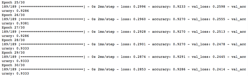
As you can see, we started with high loss (0.66) and low accuracy (0.57) on the validation set during first epoch. Gradually, we were able to decrease the loss (0.24) and improve accuracy (0.93) on the validation set on the last epoch.
Making inferences on the test set
We preprocess the previously unseen test set in a manner similar to the trainset and save it in scaled_test_samples. The corresponding labels are stored in test_labels .
predictions = model.predict(x = scaled_test_samples,
                            batch_size= 10,
                            verbose=0)
Make sure to pick exact same
batch_sizeas used in the training process.
Since our last hidden layer had a softmax activation function, the predictions include the output probabilities for both classes (on left we have the probability of class 0 (i.e. approved) and on right, class 1 (i.e. rejected).


There are a couple of ways to proceed from here. You could choose an arbitrary threshold value, say 0.7, and only if the probability of class 0 (i.e. approved) exceeds 0.7, should you choose to approve the loan application. Alternatively, you could pick the class with the highest probability as the final prediction. For instance, based on the above screenshot the model predicts a loan will be approved with a 2% probability but will be rejected with a 97% probability. Thus, the final inference should be that person’s loan is rejected. We will be doing the latter.
# get index of the prediction with the highest probrounded_pred = np.argmax(predictions, axis = 1)
rounded_pred


Saving and Loading a Keras model
To save everything from the trained model:
model.save('models/LoanOutcome_model.h7')We have essentially saved EVERYTHING from our trained model
1. the architecture (layers, no of neurons, etc)
2. weights learned
3. training configurations (optimizers, loss)
4. state of the optimizer (allows for easy retraining)
To load the model we just saved:
from tensorflow.keras.models import load_model
new_model = load_model('models/LoanOutcome_model.h7')
To save only the architecture:
json_string = model.to_json()To reconstruct a new model from previously-stored architecture:
from tensorflow.keras.models import model_from_json
model_architecture = model_from_json(json_string)
To save only the weights:
model.save_weights('weights/LoanOutcome_weights.h7')To use the weights for some other model architecture:
model2 = Sequential([
    Dense(units=16, input_shape=(1,), activation='relu'),
    Dense(units=32, activation='relu'),
    Dense(units=2, activation='softmax')
])# retrieving the saved weights
model2.load_weights('weights/LoanOutcome_weights.h7')
And there we have it. We have successfully managed to build our first ANN, train, validate and test it and also managed to save it for future use. In the next post, we will be working our way through a Convolutional Neural Network (CNN) to tackle an image classification task.
Until then :)
Time Series Analysis using Pandas in Python
towardsdatascience.com

WRITTEN BY
Data Science Enthusiast | ‘Explain like I’m five’ proponent | Ph.D. Learning Analytics | Oxford & SFU Alumni


No comments:
Post a Comment