How to Convert Pandas Dataframe to Keras RNN and Back to Pandas for Multivariate Regression Problems

 

This post provides a straightforward Python code that takes data in Pandas dataframe and outputs predictions in the same format using Keras RNN LSTM model.

The problem I encountered was rather common (I think): Taking data in a pandas dataframe format and making predictions using a time series regression model with keras RNN where I have more than one independent X (AKA features or predictors) and one dependent y. To be more precise, the problem was not to build the model, rather to convert the data from a pandas dataframe format to a format that an RNN model (in keras) requires and obtaining predictions from the keras model back as a pandas dataframe.

It felt that wherever I looked for a solution I got explanations on how RNN works or solutions for uni-variate regression problem. Hence, I will try to keep this post as concise and focused as possible. The coding here assumes that you already did all the necessary preprocessing (e.g., data cleansing, feature engineering etc.) and have a ready-for-analysis time series in a pandas dataframe format.

What you WILL NOT find here:

· Theoretical explanations

· Nice illustrations of an RNN model

· Preprocessing techniques

· A complicated or sophisticated model

There are many sources online that well explain these issues, I highly recommend to check the StackOverflow questions and Jason Brownlee’s, Machine Learning Mastery blog post.

What you WILL find here:

· A straightforward Python code that takes a pandas dataframe and outputs predictions in the same format using a keras RNN LSTM model for multivariate regression problems.

This post will describe snippets of code with explanations and a full seamless code will be provided at the end.

Let’s begin:

Step 1, let’s import all needed packages and check the keras version

As you can see, my keras version is 2.3.1, so if you have some problems with the code I post here, please check that you have the same version or a higher one.

Step 2, read the data

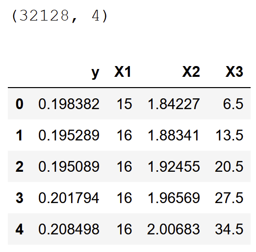
As you can see, I have 32,128 rows and four columns, with one y and three X. The code here can work on any number of X including just one X. Note that you need to define your y column in order to make things easier and more generic.

Optional step — plot the data

I know, the resolution is not great here but you get the idea of how my data looks like.

Step 3, split the data to train and test

Please note here the comment in line #3. Let’s plot again to see if our split makes sense.

Again, don’t mind the resolution, it’s not important. The plot looks good, the past (blue) is our training data and recent dates are our test data (orange).

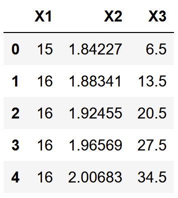
Step 4, separate X and y only for the training data. We will handle the test data later.

Now, the X_train looks like this:

and the y_train looks like this:

Step 5, scale and prepare X and y data for keras

This part requires some explanations. Here we convert the data from pandas dataframe to numpy arrays which is required by keras. In line 1–8 we first scale X and y using the sklearn MinMaxScaler model, so that their range will be from 0 to 1. The next lines are some shape manipulation to the y in order to make it applicable for keras. We need the shape of y to be (n, ), where n is the number of rows. Line 12 “pushes” the y data one step forward by adding zero in the first position and line 13 keeps the shape of y by deleting the last time step (last row). Here is a simplified example of what happens in line 12–13:

#let's say y = [1,2,3,4]
# y = np.insert(y,0,0) --> [0,1,2,3,4]
# y = np.delete(y,-1) --> [0,1,2,3]

If this is explanation is not clear enough, I refer you to Jason Brownlee’s blog post Multivariate Time Series Forecasting with LSTMs in Keras. Look for the section with the title: Multivariate Inputs and Dependent Series Example.

To sum up the shape manipulation of y let’s have a quick look on what happened. We started with y data as a dataframe:

And now it should look like this:

array([0.        , 0.12779697, 0.12401905, ..., 0.59237795, 0.6018512 , 0.61132446])

Step 6, combine X and y using the keras TimeseriesGenerator

The TimeseriesGenerator transforms the separate X and y into a structure of samples ready to train deep learning models. I would recommend to print the shape of the generator object to make sure it worked. The shape should be (batch_size,n_input,n_features)exactly how it shows in step 6 in line 8.

The hard part of converting our data from pandas dataframe to something ready to use for deep learning models is behind us. Now we can move on to step 7, instantiate the model:

Note that I used here a very simple model, with only one hidden layer and without a dropout layer. This is because I wanted to keep this post concise and the actual model architecture is not the focus here. But feel free to experiment with more layers.

Step 8, fit the model and plot the losses

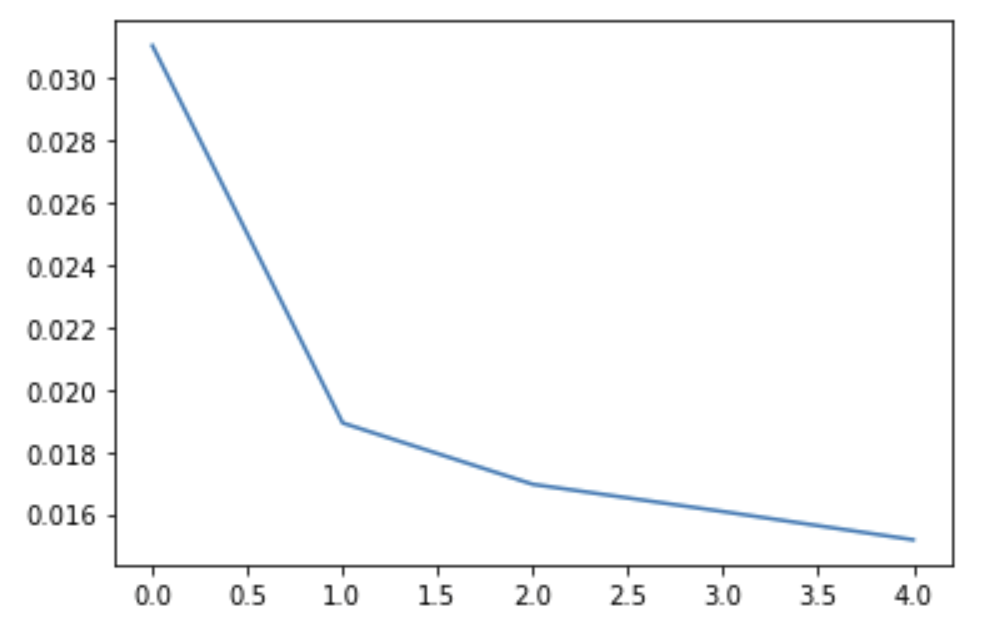
Also here, I used simple settings, only 5 epochs, just to illustrate the entire process.

Now the model is ready to use and we can make predictions on the test set.

The first line generates the X_test data by dropping the y from the test set, we do not want the y data to be included in the X. Then we scale the X_test according to the MinMaxScaler model which was fitted on the X_train earlier. Line 3 is important because we need to create a TimeseriesGenerator for the test data. I was struggling with this part because in the examples that I saw the y_test was included in here , but I do not want the model to have any knowledge whatsoever about the y_test data. I did not want the slightest chance of data leakage that will result in bias predictions. Thanks to a great help I received from Marco Cerliani on StackOverflow I understood that the second argument in the TimeseriesGenerator, which is the y_test is just a prediction method and that the actual values of the y_test don’t matter (in this specific place), so you can insert a dummy y_test → an array of zeros that has the same shape of the actual y_test data. The rest of the TimeseriesGenerator is similar to the training data, and also here I printed the shape to make sure it’s OK.

Line 10 calls the predict method and line 11 rescales the predictions. Remember that we earlier scaled the y data between 0 and 1, so we need to scale it back. In line 12 we construct a dataframe from y_true and y_pred. Note that we only call for a subset of y_true (test[y_col].values[n_input:]), this is because the model needs n_input timesteps (rows or observations) to start predict, so it takes these n_input (in this case 25 timesteps) from X_test and only then start to predict. For example, if we had 50 timesteps in our test set (or 50 rows or observations), then we will have only 25 predictions because the first 25 were used by the model according to its architecture that we set.

Now we have our results in a nice pandas dataframe structure:

And we can plot them using results.plot();:

That’s it, we began with data in a pandas dataframe format and finished with predictions in the same format.

That’s the entire code in one block

I hope this is useful and will help you in your machine learning missions. Please write me below if you have any comments.

import pandas as pd
	import numpy as np
	import keras
	import matplotlib.pyplot as plt
	from sklearn.preprocessing import MinMaxScaler
	from pandas.plotting import register_matplotlib_converters
	register_matplotlib_converters()
	from keras.preprocessing.sequence import TimeseriesGenerator
	from keras.models import Sequential
	from keras.layers import Dense
	from keras.layers import LSTM
	df = pd.read_pickle(r'C:\....\data.pkl') # read data
	y_col='y' # define y variable, i.e., what we want to predict
	test_size = int(len(df) * 0.1) # here I ask that the test data will be 10% (0.1) of the entire data
	train = df.iloc[:-test_size,:].copy() # the copy() here is important, it will prevent us from getting: SettingWithCopyWarning: A value is trying to be set on a copy of a slice from a DataFrame.
	# Try using .loc[row_index,col_indexer] = value instead
	test = df.iloc[-test_size:,:].copy()
	X_train = train.drop(y_col,axis=1).copy()
	y_train = train[[y_col]].copy() # the double brakets here are to keep the y in dataframe format, otherwise it will be pandas Series
	Xscaler = MinMaxScaler(feature_range=(0, 1)) # scale so that all the X data will range from 0 to 1
	Xscaler.fit(X_train)
	scaled_X_train = Xscaler.transform(X_train)
	Yscaler = MinMaxScaler(feature_range=(0, 1))
	Yscaler.fit(y_train)
	scaled_y_train = Yscaler.transform(y_train)
	scaled_y_train = scaled_y_train.reshape(-1) # remove the second dimention from y so the shape changes from (n,1) to (n,)
	scaled_y_train = np.insert(scaled_y_train, 0, 0)
	scaled_y_train = np.delete(scaled_y_train, -1)
	n_input = 25 #how many samples/rows/timesteps to look in the past in order to forecast the next sample
	n_features= X_train.shape[1] # how many predictors/Xs/features we have to predict y
	b_size = 32 # Number of timeseries samples in each batch
	generator = TimeseriesGenerator(scaled_X_train, scaled_y_train, length=n_input, batch_size=b_size)
	model = Sequential()
	model.add(LSTM(150, activation='relu', input_shape=(n_input, n_features)))
	model.add(Dense(1))
	model.compile(optimizer='adam', loss='mse')
	model.fit_generator(generator,epochs=5)
	X_test = test.drop(y_col,axis=1).copy()
	scaled_X_test = Xscaler.transform(X_test)
	test_generator = TimeseriesGenerator(scaled_X_test, np.zeros(len(X_test)), length=n_input, batch_size=b_size)
	y_pred_scaled = model.predict(test_generator)
	y_pred = Yscaler.inverse_transform(y_pred_scaled)
	results = pd.DataFrame({'y_true':test[y_col].values[n_input:],'y_pred':y_pred.ravel()})