What is Image Classification?
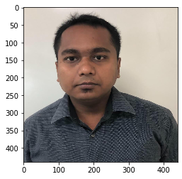
Image classification is the process of segmenting images into different categories based on their features. A feature could be the edges in an image, the pixel intensity, the change in pixel values, and many more. We will try and understand these components later on. For the time being let’s look into the images below (refer to Figure 1). The three images belong to the same individual however varies when compared across features like the color of the image, position of the face, the background color, color of the shirt, and many more. The biggest challenge when working with images is the uncertainty of these features. To the human eye, it looks all the same, however, when converted to data you may not find a specific pattern across these images easily.


An image consists of the smallest indivisible segments called pixels and every pixel has a strength often known as the pixel intensity. Whenever we study a digital image, it usually comes with three color channels, i.e. the Red-Green-Blue channels, popularly known as the “RGB” values. Why RGB? Because it has been seen that a combination of these three can produce all possible color pallets. Whenever we work with a color image, the image is made up of multiple pixels with every pixel consisting of three different values for the RGB channels. Let’s code and understand what we are talking about.
import cv2
import seaborn as sns
import matplotlib.pyplot as plt
%matplotlib inline
sns.set(color_codes=True)# Read the image
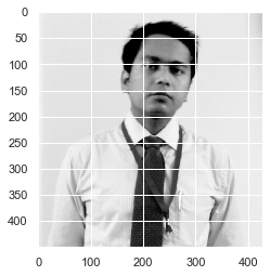
image = cv2.imread('Portrait-Image.png') #--imread() helps in loading an image into jupyter including its pixel valuesplt.imshow(cv2.cvtColor(image, cv2.COLOR_BGR2RGB))
# as opencv loads in BGR format by default, we want to show it in RGB.
plt.show()image.shape
The output of image.shape is (450, 428, 3). The Shape of the image is 450 x 428 x 3 where 450 represents the height, 428 the width, and 3 represents the number of color channels. When we say 450 x 428 it means we have 192,600 pixels in the data and every pixel has an R-G-B value hence 3 color channels.
image[0][0]image [0][0] provides us with the R-G-B values of the first pixel which are 231, 233, and 243 respectively.
# Convert image to grayscale. The second argument in the following step is cv2.COLOR_BGR2GRAY, which converts colour image to grayscale.
gray = cv2.cvtColor(image, cv2.COLOR_BGR2GRAY)
print(“Original Image:”)plt.imshow(cv2.cvtColor(gray, cv2.COLOR_BGR2RGB))
# as opencv loads in BGR format by default, we want to show it in RGB.
plt.show()gray.shape
The output of gray.shape is 450 x 428. What we see right now is an image consisting of 192,600 odd pixels but consists of one channel only.
When we try and covert the pixel values from the grayscale image into a tabular form this is what we observe.
import numpy as np
data = np.array(gray)
flattened = data.flatten()flattened.shape
Output: (192600,)
We have the grayscale value for all 192,600 pixels in the form of an array.
flattenedOutput: array([236, 238, 238, ..., 232, 231, 231], dtype=uint8). Note a grayscale value can lie between 0 to 255, 0 signifies black and 255 signifies white.
Now if we take multiple such images and try and label them as different individuals we can do it by analyzing the pixel values and looking for patterns in them. However, the challenge here is that since the background, the color scale, the clothing, etc. vary from image to image, it is hard to find patterns by analyzing the pixel values alone. Hence we might require a more advanced technique that can detect these edges or find the underlying pattern of different features in the face using which these images can be labeled or classified. This where a more advanced technique like CNN comes into the picture.
What is CNN?
CNN or the convolutional neural network (CNN) is a class of deep learning neural networks. In short think of CNN as a machine learning algorithm that can take in an input image, assign importance (learnable weights and biases) to various aspects/objects in the image, and be able to differentiate one from the other.
CNN works by extracting features from the images. Any CNN consists of the following:
- The input layer which is a grayscale image
- The Output layer which is a binary or multi-class labels
- Hidden layers consisting of convolution layers, ReLU (rectified linear unit) layers, the pooling layers, and a fully connected Neural Network
It is very important to understand that ANN or Artificial Neural Networks, made up of multiple neurons is not capable of extracting features from the image. This is where a combination of convolution and pooling layers comes into the picture. Similarly, the convolution and pooling layers can’t perform classification hence we need a fully connected Neural Network.
Before we jump into the concepts further let’s try and understand these individual segments separately.

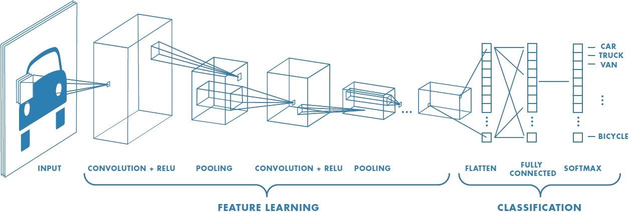
Let’s consider that we have access to multiple images of different vehicles, each labeled into a truck, car, van, bicycle, etc. Now the idea is to take these pre-label/classified images and develop a machine learning algorithm that is capable of accepting a new vehicle image and classify it into its correct category or label. Now before we start building a neural network we need to understand that most of the images are converted into a grayscale form before they are processed.
Why grayscale and not RGB/Color Images?

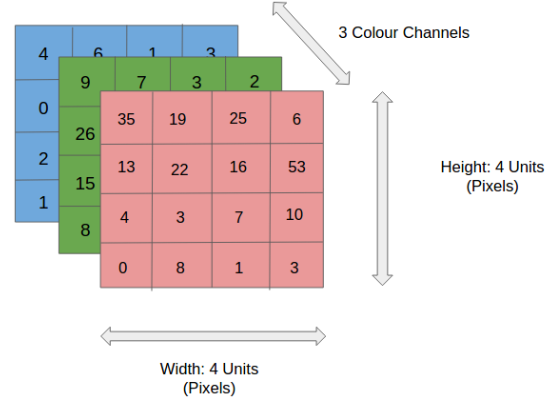
We discussed earlier that any color image has three channels, i.e. red, green, and blue as shown in Figure 3. There are several such color spaces like the grayscale, CMYK, HSV in which an image can exist.
The challenge with images having multiple color channels is that we have huge volumes of data to work with which makes the process computationally intensive. In other worlds think of it like a complicated process where the Neural Network or any machine learning algorithm has to work with three different data (R-G-B values in this case) to extract features of the images and classify them into their appropriate categories.
The role of CNN is to reduce the images into a form that is easier to process, without losing features critical towards a good prediction. This important when we need to make the algorithm scalable to massive datasets.
What are convolutions?
We understand that the training data consists of grayscale images which will be an input to the convolution layer to extract features. The convolution layer consists of one or more Kernels with different weights that are used to extract features from the input image. Say in the example above we are working with a Kernel (K) of size 3 x 3 x 1 (x 1 because we have one color channel in the input image), having weights outlined below.
Kernel/Filter, K =
1  0  1
0  1  0
1  0  1
When we slide the Kernel over the input image (say the values in the input image are grayscale intensities) based on the weights of the Kernel we end up calculating features for different pixels based on their surrounding/neighboring pixel values. E.g. when the Kernel is applied on the image for the first time as illustrated in Figure 5 below we get a feature value equal to 4 in the convolved feature matrix as shown below.


If we observe Figure 4 carefully we will see that the kernel shifts 9 times across image. This process is called Stride. When we use a stride value of 1 (Non-Strided) operation we need 9 iterations to cover the entire image. The CNN learns the weights of these Kernels on its own. The result of this operation is a feature map that basically detects features from the images rather than looking into every single pixel value.
Image features, such as edges and interest points, provide rich information on the image content. They correspond to local regions in the image and are fundamental in many applications in image analysis: recognition, matching, reconstruction, etc. Image features yield two different types of problem: the detection of the area of interest in the image, typically contours, and the description of local regions in the image, typically for matching in different images, (Image features. (n.d.))
Let’s take a deeper look into what we are talking about.
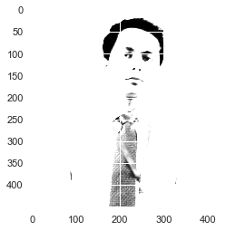
Extracting features from an image is similar to detecting edges in the image. We can use the openCV package to perform the same. We will declare a few matrices, apply them on a grayscale image, and try and look for edges. You can find more about the function here.
# 3x3 array for edge detection
mat_y = np.array([[ -1, -2, -1],
                   [ 0, 0, 0],
                   [ 1, 2, 1]])
mat_x = np.array([[ -1, 0, 1],
                   [ 0, 0, 0],
                   [ 1, 2, 1]])

filtered_image = cv2.filter2D(gray, -1, mat_y)
plt.imshow(filtered_image, cmap='gray')filtered_image = cv2.filter2D(gray, -1, mat_x)
plt.imshow(filtered_image, cmap='gray')


import torch
import torch.nn as nn
import torch.nn.functional as fn
If you are working with windows install the following — # conda install pytorch torchvision cudatoolkit=10.2 -c pytorch for using pytorch.
import numpy as np
filter_vals = np.array([[-1, -1, 1, 2], [-1, -1, 1, 0], [-1, -1, 1, 1], [-1, -1, 1, 1]])
print(‘Filter shape: ‘, filter_vals.shape)# Neural network with one convolutional layer and four filters
class Net(nn.Module):

 def __init__(self, weight): #Declaring a constructor to initialize the class variables
 super(Net, self).__init__()
 # Initializes the weights of the convolutional layer to be the weights of the 4 defined filters
 k_height, k_width = weight.shape[2:]
 # Assumes there are 4 grayscale filters; We declare the CNN layer here. Size of the kernel equals size of the filter
 # Usually the Kernels are smaller in size
 self.conv = nn.Conv2d(1, 4, kernel_size=(k_height, k_width), bias=False)
 self.conv.weight = torch.nn.Parameter(weight)

 def forward(self, x):
 # Calculates the output of a convolutional layer pre- and post-activation
 conv_x = self.conv(x)
 activated_x = fn.relu(conv_x)# Returns both layers
 return conv_x, activated_x# Instantiate the model and set the weights
weight = torch.from_numpy(filters).unsqueeze(1).type(torch.FloatTensor)
model = Net(weight)# Print out the layer in the network
print(model)
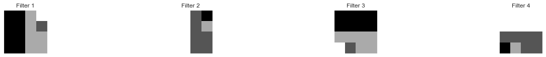
We create the visualization layer, call the class object, and display the output of the Convolution of four kernels on the image (Bonner, 2019).
def visualization_layer(layer, n_filters= 4):

    fig = plt.figure(figsize=(20, 20))

    for i in range(n_filters):
        ax = fig.add_subplot(1, n_filters, i+1, xticks=[], yticks=[])
        # Grab layer outputs
        ax.imshow(np.squeeze(layer[0,i].data.numpy()), cmap='gray')
        ax.set_title('Output %s' % str(i+1))
The convolution operation.
#-----------------Display the Original Image-------------------
plt.imshow(gray, cmap='gray')#-----------------Visualize all of the filters------------------
fig = plt.figure(figsize=(12, 6))
fig.subplots_adjust(left=0, right=1.5, bottom=0.8, top=1, hspace=0.05, wspace=0.05)for i in range(4):
    ax = fig.add_subplot(1, 4, i+1, xticks=[], yticks=[])
    ax.imshow(filters[i], cmap='gray')
    ax.set_title('Filter %s' % str(i+1))

# Convert the image into an input tensor
gray_img_tensor = torch.from_numpy(gray).unsqueeze(0).unsqueeze(1)
# print(type(gray_img_tensor))# print(gray_img_tensor)# Get the convolutional layer (pre and post activation)
conv_layer, activated_layer = model.forward(gray_img_tensor.float())# Visualize the output of a convolutional layer
visualization_layer(conv_layer)
Output:


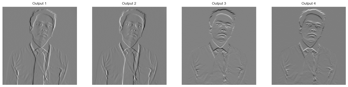
Note: Depending on the weights associated with a filter, the features are detected from the image. Notice when an image is passed through a convolution layer, it and tries and identify the features by analyzing the change in neighboring pixel intensities. E.g. the top right of the image has similar pixel intensity throughout, hence no edges are detected. It is only when the pixels change intensity the edges are visible.
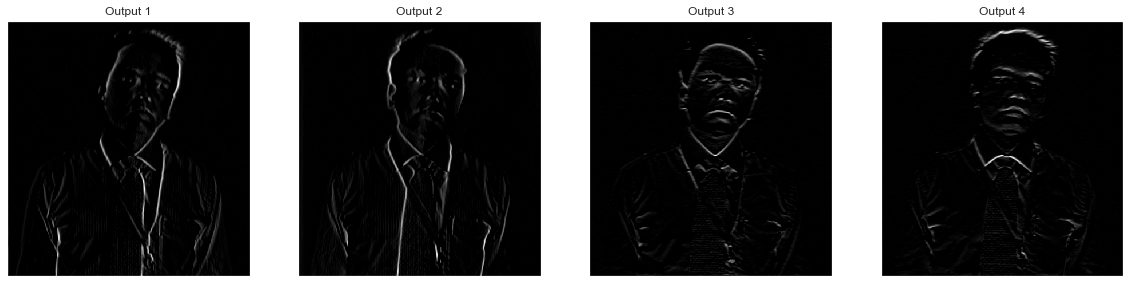
Why ReLU?
ReLU or rectified linear unit is a process of applying an activation function to increase the non-linearity of the network without affecting the receptive fields of convolution layers. ReLU allows faster training of the data, whereas Leaky ReLU can be used to handle the problem of vanishing gradient. Some of the other activation functions include Leaky ReLU, Randomized Leaky ReLU, Parameterized ReLU Exponential Linear Units (ELU), Scaled Exponential Linear Units Tanh, hardtanh, softtanh, softsign, softmax, and softplus.
visualization_layer(activated_layer)


The general objective of the convolution operation is to extract high-level features from the image. We can always add more than one convolution layer when building the neural network, where the first Convolution Layer is responsible for capturing gradients whereas the second layer captures the edges. The addition of layers depends on the complexity of the image hence there are no magic numbers on how many layers to add. Note application of a 3 x 3 filter results in the original image results in a 3 x 3 convolved feature, hence to maintain the original dimension often the image is padded with values on both ends.
Role of the Pooling Layer
The pooling layer applies a non-linear down-sampling on the convolved feature often referred to as the activation maps. This is mainly to reduce the computational complexity required to process the huge volume of data linked to an image. Pooling is not compulsory and is often avoided. Usually, there are two types of pooling, Max Pooling, that returns the maximum value from the portion of the image covered by the Pooling Kernel and the Average Pooling that averages the values covered by a Pooling Kernel. Figure 12 below provides a working example of how different pooling techniques work.

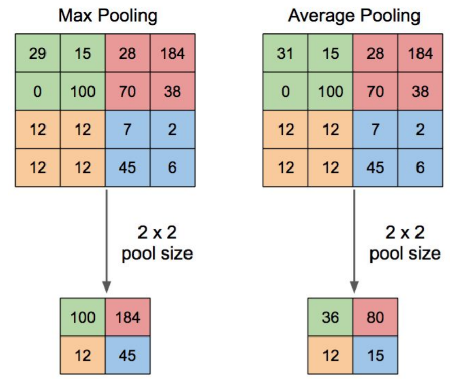
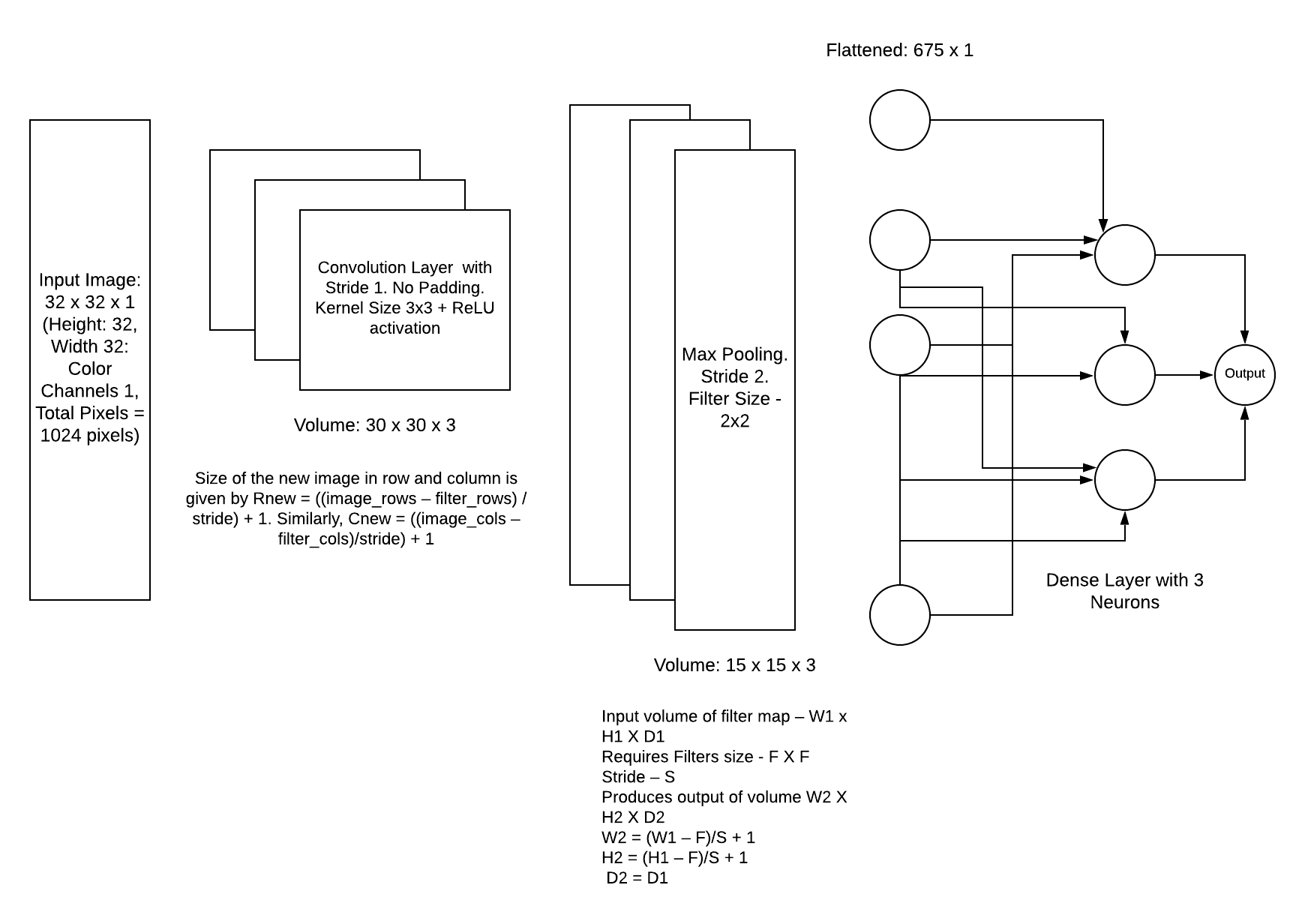
Image Flattening
Once the pooling is done the output needs to be converted to a tabular structure that can be used by an artificial neural network to perform the classification. Note the number of the dense layer as well as the number of neurons can vary depending on the problem statement. Also often a drop out layer is added to prevent overfitting of the algorithm. Dropouts ignore few of the activation maps while training the data however use all activation maps during the testing phase. It prevents overfitting by reducing the correlation between neurons.

Working with the CIFAR-10 dataset
An end to end example of working with CNN using Keras is provided in the link below.
Reference
- Saha, S. (2018). A Comprehensive Guide to Convolutional Neural Networks — the ELI5 way. [online] Towards Data Science. Available at: https://towardsdatascience.com/a-comprehensive-guide-to-convolutional-neural-networks-the-eli5-way-3bd2b1164a53.
- Image features. (n.d.). [online] Available at: http://morpheo.inrialpes.fr/~Boyer/Teaching/Mosig/feature.pdf.
- Stanford Univeristy (2018). Introduction to Convolutional Neural Networks. [online] Available at: https://web.stanford.edu/class/cs231a/lectures/intro_cnn.pdf.
- Visin, V.D., Francesco (2016). English: Animation of a variation of the convolution operation. Blue maps are inputs, and cyan maps are outputs. [online] Wikimedia Commons. Available at: https://commons.wikimedia.org/wiki/File:Convolution_arithmetic_-_Same_padding_no_strides.gif [Accessed 20 Aug. 2020].
- Bonner, A. (2019). The Complete Beginner’s Guide to Deep Learning: Convolutional Neural Networks. [online] Medium. Available at: https://towardsdatascience.com/wtf-is-image-classification-8e78a8235acb.
About the Author: Advanced analytics professional and management consultant helping companies find solutions for diverse problems through a mix of business, technology, and math on organizational data. A Data Science enthusiast, here to share, learn and contribute; You can connect with me on Linked and Twitter;


No comments:
Post a Comment