Beginners usually ignore most foundational statistical knowledge. To understand different models, and various techniques better, these concepts are essential. These work as baseline knowledge for various concepts involved in data science, machine learning, and artificial intelligence.
Here is the list of concepts covered in this article.
- Measures of central tendency
- Measures of spread
- Population & sample
- Central limit theorem
- Sampling & sampling techniques
- Selection Bias
- Correlation & various correlation coefficients
Let’s dive in!


1 — Measures of central tendency
A measure of central tendency is a single value that attempts to describe a set of data by identifying the central position within that set of data. The three most common values used as a measure of center are,
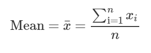
— Mean is the average of all the values in data.

— Median is the middle value in the sorted(ordered) data. Median is a better measure of center than mean as it is not affected by outliers.
— Mode is the most frequent value in the data.
2 — Measures of spread
Measures of spread describe how similar or varied the set of observed values are for a particular variable (data item). Measures of spread include the range, quartiles, and the interquartile range, variance, and standard deviation.
— Range is the difference between the smallest value and the largest value in the data.
— Quartiles divide an ordered dataset into four equal parts, and refer to the values of the point between the quarters.
The lower quartile (Q1) is the value between the lowest 25% of values and the highest 75% of values. It is also called the 25th percentile.
The second quartile (Q2) is the middle value of the data set. It is also called the 50th percentile, or the median.
The upper quartile (Q3) is the value between the lowest 75% and the highest 25% of values. It is also called the 75th percentile.

The interquartile range (IQR) is the difference between the upper (Q3) and lower (Q1) quartiles, and describes the middle 50% of values when ordered from lowest to highest. The IQR is often seen as a better measure of spread than the range as it is not affected by outliers.
— The variance of all the data points whose mean is μ, each data point is denoted by Xi, and N number of data points is given by,

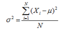
The standard deviation is the square root of the variance. The standard deviation for a population is represented by σ.
In datasets with a small spread, all values are very close to the mean, resulting in a small variance and standard deviation. Where a dataset is more dispersed, values are spread further away from the mean, leading to a larger variance and standard deviation.
3 — Population and Sample
- The population is the entire set of possible data values.
- A sample of data set contains a part, or a subset, of a population. The size of a sample is always less than the size of the population from which it is taken.


For example, the set of all people of a country is ‘population’ and a subset of people is ‘sample’ which is usually less than the population.
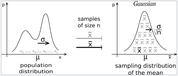
4 — Central Limit Theorem
Central Limit Theorem is a key concept in probability theory because it implies that probabilistic and statistical methods that work for normal distributions can be applicable to many problems involving other types of distributions.
CLT states that, “Sampling from a population using a sufficiently large sample size, the mean of the samples, known as the sample mean, will be normally distributed. This is true regardless of the distribution of the population.”

Other acumens from CLT are,
- The sample mean converges in probability and almost surely to the expected value of the population mean.
- The variance of the population is the same as the product of variance of the sample and the number of elements in each sample.
5— Sampling & Sampling techniques
Sampling is a statistical analysis technique used to select, manipulate, and analyze a representative subset of the data points to identify patterns and trends in the larger data set under observation.
There are many different methods for drawing samples from the data; the ideal one depends on the data set and problem in hand. Commonly used sampling techniques are given below,
- Simple random sampling: In this case, each value in the sample is chosen entirely by chance and each value of the population has an equal chance, or probability, of being selected.
- Stratified sampling: In this method, the population is first divided into subgroups (or strata) which share a similar characteristic. It is used when we might reasonably expect the measurement of interest to vary between the different subgroups, and we want to ensure representation from all the subgroups.
- Cluster sampling: In a clustered sample, subgroups of the population are used as the sampling unit, rather than individual values. The population is divided into subgroups, known as clusters, which are randomly selected to be included in the study.
- Systematic sampling: Individual values are selected at regular intervals from the sampling frame. The intervals are chosen to ensure an adequate sample size. If you need a sample size n from a population of size x, you should select every x/nth individual for the sample.
6 — Selection Bias
Selection bias (also called Sampling bias) is a systematic error due to a non-random sample of a population, causing some values of the population to be less likely to be included than others, resulting in a biased sample, in which all values are not equally balanced or objectively represented.
This means that proper randomization is not achieved, thereby ensuring that the sample obtained is not representative of the population intended to be analyzed.
In the general case, selection biases cannot be overcome with statistical analysis of existing data alone. An assessment of the degree of selection bias can be made by examining correlations.
7 — Correlation
Correlation is simply, a metric that measures the extent to which variables (or features or samples or any groups) are associated with one another. In almost any data analysis, data scientists will compare two variables and how they relate to one another.
The following are the most widely used correlation techniques,
- Covariance
- Pearson Correlation Coefficient
- Spearman Rank Correlation Coefficient
1. Covariance
For two samples, say, X and Y, let E(X), E(Y) be the mean values of X, Y respectively, and ‘n’ be the total number of data points. The covariance of X, Y is given by,

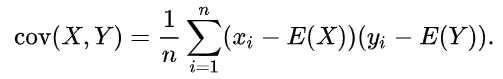
The sign of the covariance indicates the tendency of the linear relationship between the variables.


2. Pearson Correlation Coefficient
Pearson Correlation Coefficient is a statistic that also measures the linear correlation between two features. For two samples, X, Y let σX, σY be the standard deviations of X, Y respectively. PCC of X, Y is given by,


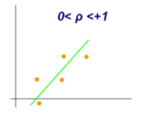
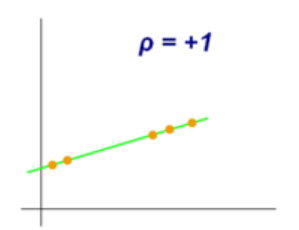
It has a value between -1 and +1.


3. Spearman Rank Correlation Coefficient
Spearman Rank Correlation Coefficient (SRCC) assesses how well the relationship between two samples can be described using a monotonic function (whether linear or not) where PCC can assess only linear relationships.
The Spearman rank correlation coefficient between the two samples is equal to the Pearson correlation coefficient between the rank values of those two samples. Rank is the relative position label of the observations within the variable.
Intuitively, the Spearman rank correlation coefficient between two variables will be high when observations have a similar rank between the two variables and low when observations have a dissimilar rank between the two variables.
The Spearman rank correlation coefficient lies between +1 and -1 where
- 1 is a perfect positive correlation
- 0 is no correlation
- −1 is a perfect negative correlation
To know more about correlation techniques and when to which one, do check that article below.
Thanks for the read. I am going to write more beginner-friendly posts in the future too. Follow me up on Medium to be informed about them. I welcome feedback and can be reached out on Twitter ramya_vidiyala and LinkedIn RamyaVidiyala. Happy learning!


No comments:
Post a Comment