Linear Regression Model for Machine Learning

 

An overview of the oldest supervised machine-learning algorithm, its type & shortcomings.

Linear Regression is one of the fundamental supervised-machine learning algorithm. While it is relatively simple and might not seem fancy enough when compared to other Machine Learning algorithms, it remains widely used across various domains such as Biology, Social Sciences, Finance, Marketing. It is extremely powerful and can be used to forecast trends or generate insights.Thus, I simply cannot emphasize enough how important it is to know Linear Regression — its working and variants — inside out before moving on to more complicated ML techniques.

---

Linear Regression Models are extremely powerful and can be used to forecast trends & generate insights.

---

The objective of the article is to provide a comprehensive overview of linear regression model. It will serve as an excellent guide for last-minute revisions or to develop a mindmap for studying Linear Regression in detail.

Note: Throughout this article, we will work with the popular Boston Housing Dataset which can be imported directly in Python using sklearn.datasets or in R using the library MASS(Modern Applied Statistics Functions). The code chunks are written in R.

What is Linear Regression?

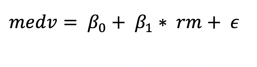
Linear Regression is a statistical/machine learning technique that attempts to model the linear relationship between the independent predictor variables X and a dependent quantitative response variable Y. It is important that the predictor and response variables be numerical values. A general linear regression model can be represented mathematically as

Linear Regression Model Equation; Image by Author

Since the linear regression model approximates the relationship between Y and X, by capturing the irreducible error term we get

Linear Regression Model Equation with Approximation; Image by Author

Here, we will use Linear Regression to predict Median House Value (Y/response variable = medv)for 506 neighborhoods around Boston.

What insights does Linear Regression reveal?

Using Linear Regression to predict median house values will help answer the following five questions:

1. Is there a linear relationship between the predictor & response variables?
2. Is there an association between the predictor & response variables? How strong?
3. How does each predictor variable effect the response variable?
4. How accurate is the prediction of response variable?
5. Is there any interaction among the independent variable?

Types of Linear Regression Model

Depending on the number of predictor variables, Linear Regression can be classified into two categories:

1. Simple Linear Regression — One predictor variable.
2. Multiple Linear Regression — Two or more predictor variables.

The simplicity of linear regression model can be attributed to its core assumptions. However, these assumptions introduce bias in the model which leads to over-generalization/under-fitting (More about Bias-Variance Tradeoff).

---

An easy to remember acronym for the assumption of Linear Regression Model is LINE

---

Assumptions of Linear Regression Model

LINE — a simple acronym that captures the four assumptions of Linear Regression Model.

1. Linear Relationship: The relationship between predictor & response variable is linear.
2. Independent Observations: Observations in the dataset are independent of each other.
3. Normal distribution of residuals.
4. Errors/Residuals have a constant variance: Also known as Homoscedasticity.

Simple Linear Regression

A simple learning regression model predicts the response variable Y using a single predictor variable X. For the Boston Housing Dataset, post analyzing the correlation between Median House Value / medv column and the 12 predictor columns, scatterplot of medv with a few correlated column in shown below:

Figure 1: Scatterplot for Boston Housing Dataset; Image by Author

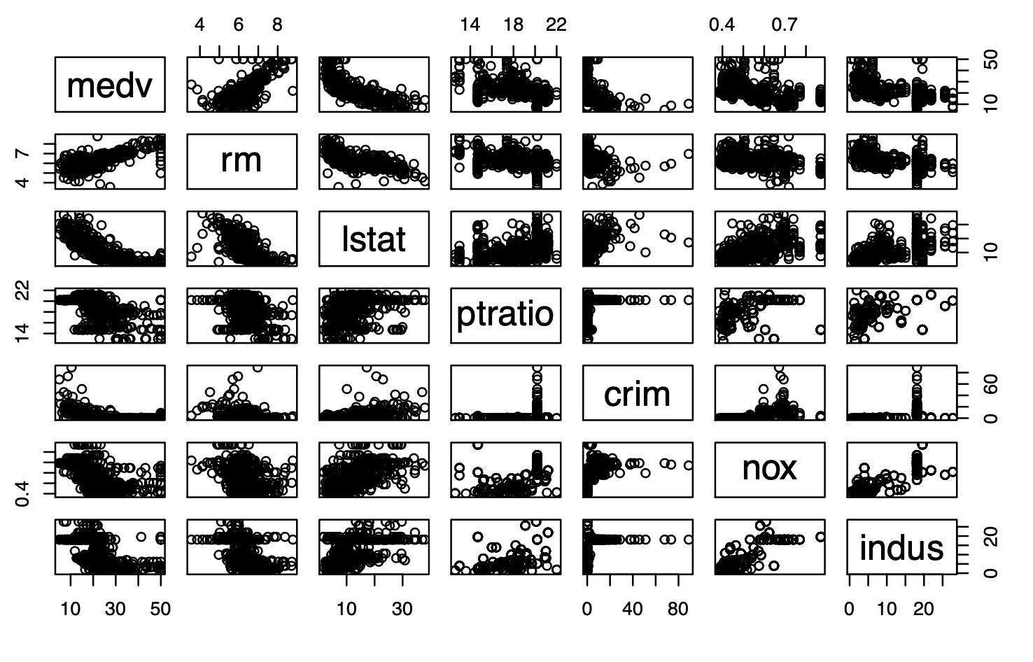
On observing the scatterplots, we notice that medv and rm (average number of rooms) have an almost linear relationship. Therefore, their relationship can be represented as

Median Price Prediction Generalized Equation; Image by Author

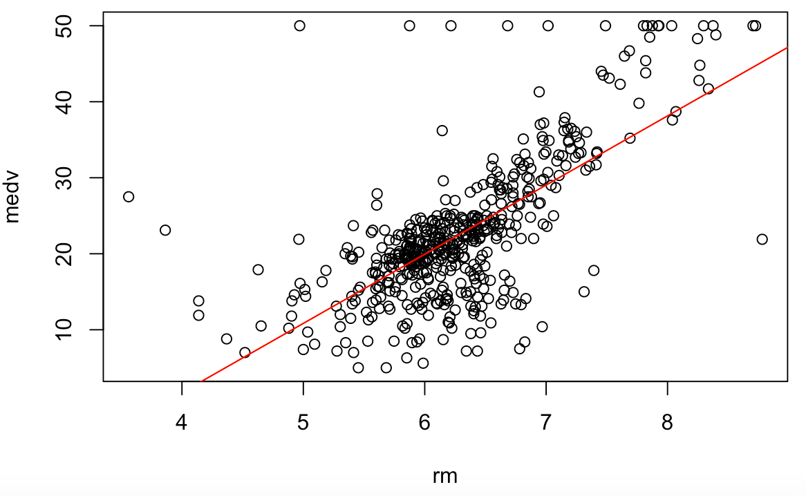
The goal is to fit a linear model by estimating the coefficients that fits as close to the 506 datapoints as possible. The difference between the predicted and the observed value is the error which needs to be minimized to find best fit. A common approach used in minimizing the least squares of errors is known as Ordinary Least Squares (OLS) method.

To create a simple linear regression model in R, run the following code chunk:

simpleLinearModel <- lm(medv ~ rm, data = Boston)

Let’s look at the fitted model,

plot(rm ,medv)
abline(simpleLinearModel, col = ‘red’)

Figure 2: Simple Linear Regression Line fitted to the training data; Image by Author

---

Assess the Linear Regression Model’s accuracy using RSE, R², adjusted R², F-statistic.

---

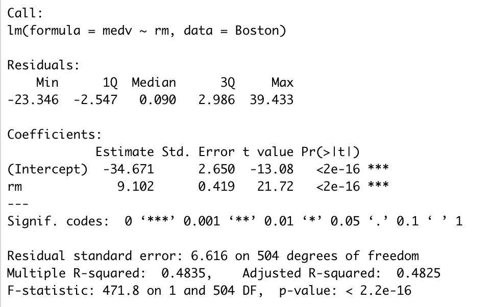
The summary of the model (Image below) tells us about the coefficient and helps in assessing the accuracy of the model using metrics such as

• Residual Standard Error (RSE)
• R² Statistic
• Adjusted R-squared
• F-statistic

which quantify how well the model fits the training data.

print(summary(simpleLinearModel))

Figure 3: Summary of Simple Linear Regression Model; Image by Author

---

How to interpret Simple Linear Regression Model?

Using Simple Linear Regression to predict median house values we can answer the following:

• Is there an association between rm & medv? How strong?

The association between medv and rm and its strength can be determined by observing the p-value corresponsing to the F-statistic in the Summary Table (Figure 3). As the p-value is very low, there is a strong association between medv and rm.

• How does rm effect medv?

According to this simple linear regression model, unit increase in the number of rooms leads to a $9.102k increase in median house value.

• How accurate is the prediction of response variable?

The RSE estimates the standard deviation of medv from the real regression line and this is only 6.616 but indicates an error of roughly ~30%. On the other hand, R² shows that only 48% variablity in medv is explained by rm. The adjusted R² & F-statistic are useful metric for multiple linear regression.

• Is there a linear relationship between the Median House Value (medv) & the number of rooms in the house (rm)?

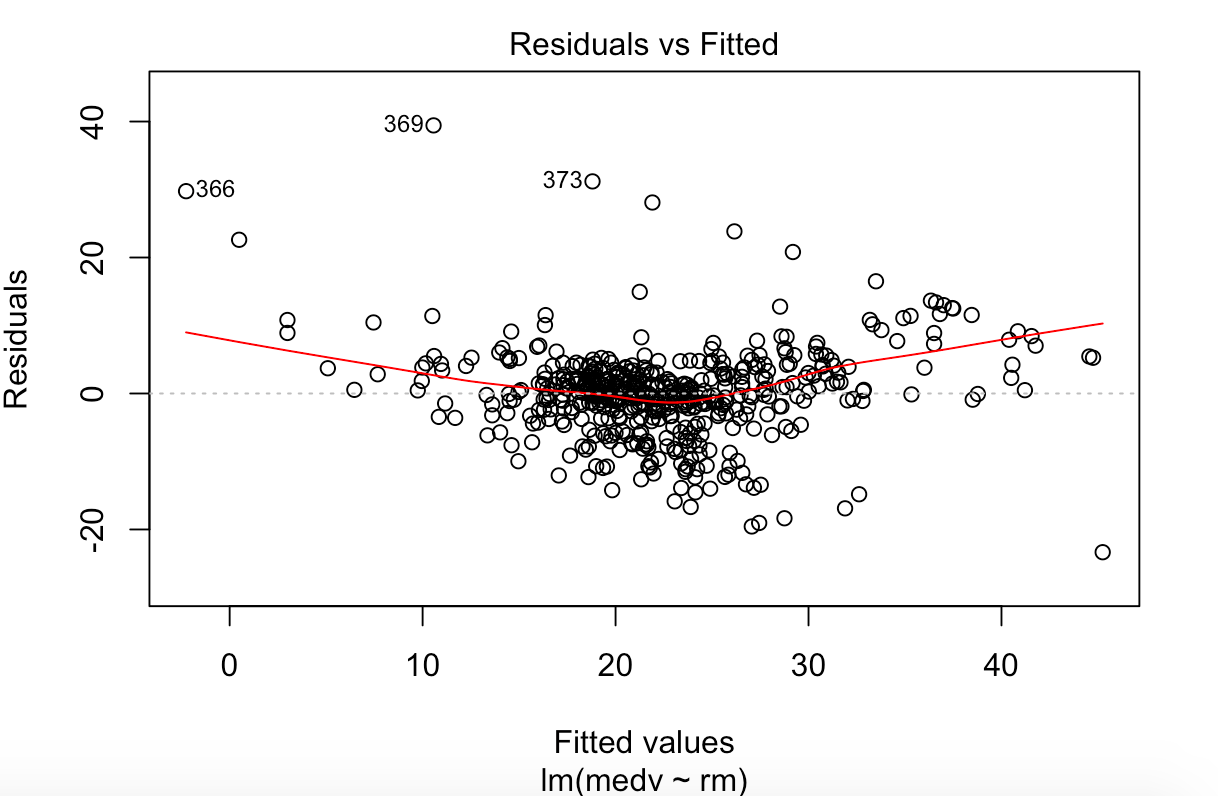
Other than using Figure 1 to identify an almost linear relationship between medv & rm, residual plots as shown in Figure 3, help idenitfy linearity, if there is no pattern present. As there is a little pattern, it indicates that there is a non-linearity component in the relationship albeit a little weak.

Figure 4: Residual plot with a smooth line to identify trend; Image by Author

Multiple Linear Regression

Multiple Linear Regression Model attempts to model a linear relationship between two or more predictor variables and a response variable. The most important question that comes to one’s mind is

“How to choose predictor variables which are useful?”

This is known as Regression Variable Selection can be acheived by using:

1. Best Subset Selection
2. Stepwise Selection — Forward, Backward, Hybrid

There are plenty of other ways to acheive this. By using Forward Stepwise Selection, I found that all predictor variables except age and indus are important for predicting medv.

#Variable selection using stepwise regression
nullmodel <- lm(medv ~ 1, data = Boston)
fullmodel <- lm(medv ~ ., data = Boston)#Forward Stepwise Selection
mulitpleLinearModel <- step(nullmodel, scope = list(lower = nullmodel, upper = fullmodel), direction = "forward")

How to interpret Multiple Linear Regression Model?

Using Simple Linear Regression to predict median house values we can answer the following questions using the summary of the model:

Figure 5: Summary of Multiple Linear Regression Model; Image by Author

• Is there an association between the subset of predictor variables & medv? How strong?

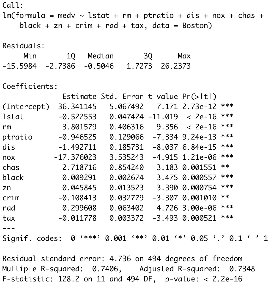
As the p-value corresponsing to the F-statistic in the Summary Table (Figure 5) is very low, there is a strong association between the subset of predictor variables & medv.

• How do the various predictor variable effect medv?

According to this multiple linear regression model, each predictor variable has a strong association with medv and the exact contribution can be discerned by using simple linear models.

• How accurate is the prediction of response variable?

The adjusted R² penalizes additional predictor variables which are added to the model and don’t improve it as opposed to R² which increases with every variable that is added to the model. Since the difference between the two is not much, we can deduce that this model is more accurate than the simple linear regression model which could explain only 48% variability in medv as opposed to 74% which can be explained by multiple linear regression.

Potential Problems with Linear Regression Model

Having looked at Linear Regression Models, its types and assessment, it is important to acknowledge its shortcomings. Due to the assumptions of the linear regression model, there are several problems which plague Linear Regression Models such as:

1. Collinearity (How to handle multi-collinearity)
2. Correlation of residuals
3. Non-constant variance/ heteroscedasticity of residuals
4. Outliers
5. Non-linear relationship

Article on how to deal with these issues is in the pipeline.

---

Projects on Github exploring simple/multiple/polynomial linear regression, non-linear transformation of predictors, stepwise selection:

1. Boston Housing Price Prediction
2. Fuel Efficiency Prediction (autompg)
3. Predicting Wages

---

References

Introduction to Statistical Learning in R by Gareth James, Daniela Witten, Trevor Hastie, Robert Tibshirani.