The idea to write this paper came to me after reading an interesting book entitled: “Machine Learning and Security” by Clarence Chio and David Freeman, published by O’Reilly Media, Inc., 2018.
The purpose of this paper is to show how much is easy and productive to develop machine learning applications using Oracle Autonomous Database and its collaborative environment for ML notebooks, based on Apache Zeppelin, in the hypothesis of developing a Network Traffic Analysis algorithm as a network attacks classifier, following the approach described in chapter 5 of the book and using the same dataset.
I will not go into too much details in the description of the Oracle Autonomous DB platform and the related Oracle Machine Learning (OML) environment, based on the PL/SQL language and the algorithms packaged in DBMS_DATA_MINING: for details refer to other papers like “Oracle Autonomous Data Warehouse Cloud Service (ADW), Part 7: Run Notebooks with Oracle Machine Learning” or others of the series dedicated to Oracle Autonomous DB.
The Dataset Import and Preparation
The dataset used for building a network intrusion detection classifier is the classic KDD you can download here, released as first version in the 1999 KDD Cup, with 125.973 records in the training set. It was built for DARPA Intrusion Detection Evaluation Program by MIT Lincoln Laboratory. It provides a raw tcpdump traffic coming from a local area network (LAN) that holds, as reported here, normal traffic and attacks falling into four main categories:
- DOS: denial-of-service;
- R2L: unauthorized access from a remote machine;
- U2R: unauthorized access to local superuser (root) privileges;
- Probing: surveillance.
The dataset is already split into training and test dataset.
The sub-classes into training dataset are 22 for attacks, and one “normal” for traffic allowed. The list of attacks and the associations with the four categories reported above is hold in this file.
In the test dataset we find 37 kind of attacks, so we have to delete records with class types not included into training set to avoid to affect the quality of final test of model accuracy.
Let’s describe how to import into an Autonomous DB instance these three main files: training/test dataset and dictionary, and analyze and prepare to provide finally to the algorithm chosen to be trained.
Oracle Cloud Infrastructure offers an Object Storage Service in which we can upload files and get an URL to set in our notebook and execute the import. In this way you have a secure and managed environment to store datasets that will be used by data scientists, without losing the governance of a datalab. Into the OCI console look for the Object Storage page as shown here:

Oracle Cloud Infrastructure console
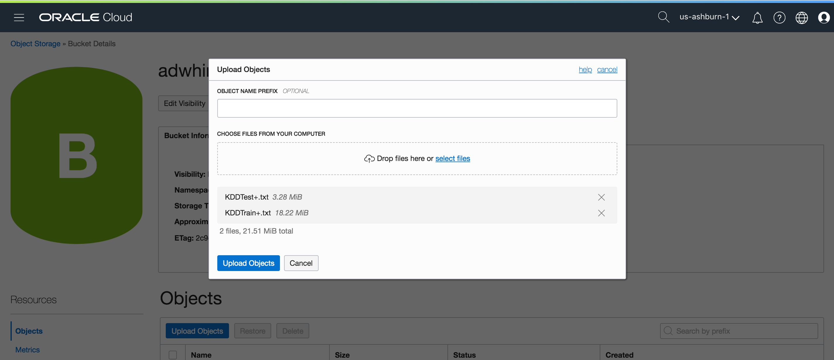
and upload the files: training_attack_types, KDDTest+.txt, KDDTrain+.txt previously downloaded using the url links reported above:
You can view the details of file uploaded and a preview of its content:
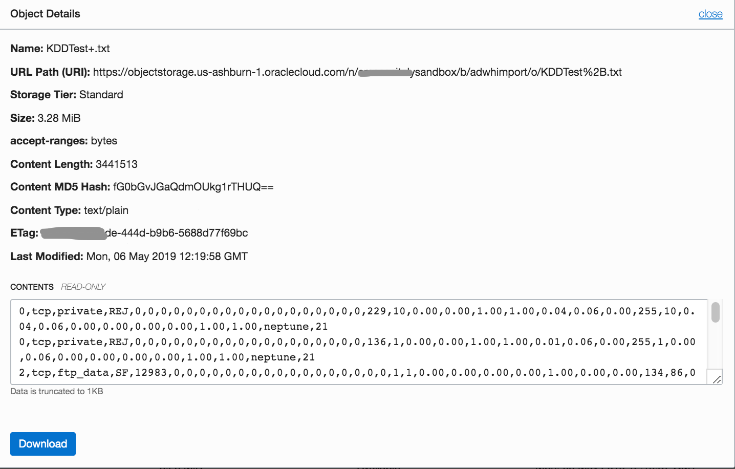
Now that your files are in the Object Storage, you need to grant the permissions to allow the import in your notebook.
In order to do this, you have to generate a token you will use in the API call. From OCI console:

Select your profile in order to access to your “Identity/Users/User Details” administration page. In this page, click on menu “Resources/Auth Tokens” in the left-down corner of the page:
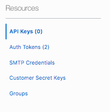
In this way you will able to generate a token you will provide as credential to access your object storage files from PL/SQL notebook.
Create a new notebook and, as your first paragraph, you can put something like this:
%scriptBEGIN
DBMS_CLOUD.DROP_CREDENTIAL(credential_name => ‘CRED_KDD’);
DBMS_CLOUD.CREATE_CREDENTIAL(
   credential_name => ‘CRED_KDD’, — Credential Token
   username => ‘oracleidentitycloudservice/email@domain.com’,
   password => ‘***************’ — Auth Token
);END;
where you have to set:
- a credential named “CRED_KDD”, that you’ll use later to get files;
- your user name ‘oracleidentitycloudservice/email@domain.com’ that you’ll find in “Identity/Users/User Details” administration page
- the auth token ‘*********************’ generated before.
Differently from pandas.read_csv(), you have to prepare a table corresponding to the file you are going to import from Object Storage. To avoid any problem during the import, I suggest to use Number type for continuos field and VARCHAR2(4000) type for categorical field.
This is the paragraph for that:
%sql
create table kdd_train (
   duration NUMBER,
   protocol_type VARCHAR2(4000),
   service VARCHAR2(4000),
   flag VARCHAR2(4000),
   src_bytes NUMBER,
   dst_bytes NUMBER,
   land VARCHAR2(4000),
   wrong_fragment NUMBER,
   urgent NUMBER,
   hot NUMBER,
   num_failed_logins NUMBER,
   logged_in VARCHAR2(4000),
   num_compromised NUMBER,
   root_shell NUMBER,
   su_attempted NUMBER,
   num_root NUMBER,
   num_file_creations NUMBER,
   num_shells NUMBER,
   num_access_files NUMBER,
   num_outbound_cmds NUMBER,
   is_host_login NUMBER,
   is_guest_login NUMBER,
   count NUMBER,
   srv_count NUMBER,
   serror_rate NUMBER,
   srv_serror_rate NUMBER,
   rerror_rate NUMBER,
   srv_rerror_rate NUMBER,
   same_srv_rate NUMBER,
   diff_srv_rate NUMBER,
   srv_diff_host_rate NUMBER,
   dst_host_count NUMBER,
   dst_host_srv_count NUMBER,
   dst_host_same_srv_rate NUMBER,
   dst_host_diff_srv_rate NUMBER,
   dst_host_same_src_port_rate NUMBER,
   dst_host_srv_diff_host_rate NUMBER,
   dst_host_serror_rate NUMBER,
   dst_host_srv_serror_rate NUMBER,
   dst_host_rerror_rate NUMBER,
   dst_host_srv_rerror_rate NUMBER,
   type VARCHAR2(4000),
   nil number
);
The last field “nil” is an improvement that will be ignored and deleted after the import. NOTE: if the import command will not find the same number of fields defined into the table, the process will be aborted.
Normally we have a full dataset and we want to split in 70%–30% proportions to get a training/test dataset. In sklearn we have a function to do this sklearn.model_selection.train_test_split(). In PL/SQL, we can simply do:
%sqlcreate table train_data as select * from dataset_table sample (70) seed (1);create table test_data as select * from dataset_table minus select * from train_data;
With the first one we’ll extract randomly 70% of dataset_table with a seed and we put into a train_data table. Then we’ll get the difference between full dataset and training dataset to create the test_data table.
The same structure it will be used for the test dataset, so we simply do a paragraph with:
%sql
CREATE TABLE kdd_test AS (SELECT * FROM kdd_train);
Now it’s time to import the datasets with DBMS_CLOUD.COPY_DATA():
DBMS_CLOUD.COPY_DATA(
  table_name =>’KDD_TRAIN’,
  credential_name =>’CRED_KDD’,
—- https://objectstorage.us-ashburn-1.oraclecloud.com/n/italysandbox/b/adwhimport/o/KDDTrain%2B.txt
  file_uri_list =>’https://swiftobjectstorage.us-ashburn-1.oraclecloud.com/v1/italysandbox/adwhimport/KDDTrain%2B.txt',
format => json_object(‘delimiter’ value ‘,’));
the main parameters to set are:
- table_name : the table previously created to import the dataset (KDD_TRAIN)
- credential_name: the key corresponding to the credential stored (CRED_KDD)
- format: set the delimiter into the file it will be imported
- file_uri_list: from the object details page, get the URL Path (URI). For example:
https://objectstorage.us-ashburn-1.oraclecloud.com/n/italysandbox/b/adwhimport/o/KDDTrain%2B.txt
and create a swift object url as follow:

At this point you can start the data exploration. For example, with this paragraph:
%sql
select distinct type, count(type) as items from kdd_train group by type
you can have the distribution of attacks type as table:

but, differently from a Python scikit-learn stack, you don’t have to write any line of codes to get a graph with matplotlib.pyplot(), but clicking on one of the icons of graphic type, you will have:

and refine the content of diagram working on “setting”, as follows:
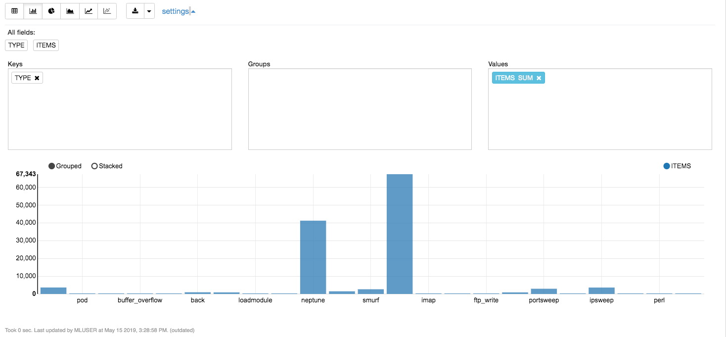
Other manipulation you can do, is dropping the “nil” field imported but not useful for training, or add a key id that isn’t into the original dataset imported:
%script
ALTER TABLE kdd_train DROP COLUMN NIL;
ALTER TABLE kdd_train ADD id number;
UPDATE kdd_train SET id = ROWNUM;
For the unbalanced distribution of this dataset, we’ll aggregate the original 23 types of records into the five categories mapped by training_attack_types file. To do this, we import as done before the file into a prepared KDD_ATTACKTYPE table, adding a record at the end to cover the “normal”traffic type:
%script
insert into KDD_ATTACKTYPE (attack,category) values (‘normal’,’normal’);
we can check the number of classes with:
%sql
select count(*) from kdd_attacktype order by attack
Now, with a simple piece of code we can manipulate the attack type reducing from 23 to 5 the classes, leveraging the dictionary created with the previous import:
%sql
UPDATE kdd_train
SET type = (
     SELECT category
     FROM kdd_attacktype
     WHERE type=attack)
WHERE type <> ‘normal’;
In this way the training dataset will hold the network traffic classified into 5 types only (one as “normal”). Now the distribution isn’t still optimal, but a bit more balanced:

That’s all: we can proceed to the training phase.
But, probably someone of you is asking if I’m missing something in the data preparation pipeline.
For example, the transformation of symbolic fields in a one-hot encoding, avoiding to leave the original field to prevent multicollinearity. Another must to have in the data preparation is the standardization process, in order to rescale the numeric fields to have a mean of 0 and a standard deviation of 1.
The replacement of missing values with the mean in case of numerical attributes or mode in case of categorical attributes, it’s another operation that if missed it could abort the training process if you use some kind of algorithms. The binning it’s another manipulation needed by algorithms like Naive Bayes.
Nothing of these manipulations are needed using Oracle Machine Learning algorithms.
The algorithms implemented on OML have the Automatic Data Preparation features that automatically does all the operations described above and much more. More details about this feature are reported here. For who wants to disable this features, it is always possible, setting the attributes of the algorithm chosen.
The Training
The phase of model training consists into a table preparation in which you’ll set the hyper-parameters you intend to set overriding the default values. In any case we have to set at least one: the algorithm name!
This is what I’ve done in the first and second execute in this paragraph:
%scriptBEGINEXECUTE IMMEDIATE ‘CREATE TABLE KDD_BUILD_SETTINGS (SETTING_NAME VARCHAR2(30), SETTING_VALUE VARCHAR2(4000))’;EXECUTE IMMEDIATE ‘INSERT INTO KDD_BUILD_SETTINGS (SETTING_NAME, SETTING_VALUE) VALUES (‘’ALGO_NAME’’,’’ALGO_DECISION_TREE’’)’;EXECUTE IMMEDIATE ‘CALL DBMS_DATA_MINING.CREATE_MODEL(‘’KDD_CLASS_MODEL’’,’’CLASSIFICATION’’,’’KDD_TRAIN’’,’’ID’’,’’TYPE’’,’’KDD_BUILD_SETTINGS’’)’;END;
In this example I’ve chosen the Decision Tree as used into the book I’ve read. In case of classification, you can use following algorithms:
- Decision Tree
- Explicit SemanticAnalysis
- Naive Bayes
- GeneralizedLinear Models(GLM)
- Random Forest
- Support Vector Machines (SVM)
- Neural Network
To “fit” the model, as you would do in sklearn, you have to call the dbms_data_mining.creat_model() API:

In OML you need to have a key_id for each record in the training dataset, for this reason I’ve simply set the rownum in a new id field during the data preparation phase.
Test and evaluation phase
In order to test the model trained, we have to convert the 37 classes in the test dataset file in the 5 classes on which it has been done the training. For the classes that aren’t in the dictionary (only 22 classes coming from training dataset), we’ll automatically find a NULL value. We’ll remove all records with NULL class to avoid an inaccurate model evaluation.
We’ll do these activities through:
%sql
UPDATE kdd_test
SET type = (SELECT category
            FROM kdd_attacktype
            WHERE type=attack)
WHERE type <> ‘normal’;
and:
%script
DELETE FROM KDD_TEST where type is NULL;
Now we are ready to check the accuracy of network traffic classification model. There are several ways. In this case we use the apply() API in order to compute the Confusion Matrix that’s useful to test the quality of a classification model.
This is the code to do that:
%scriptbegin
declare
  v_accuracy NUMBER;
begin
   DBMS_DATA_MINING.APPLY(
     model_name => ‘KDD_CLASS_MODEL’,
     data_table_name => ‘KDD_TEST’,
     case_id_column_name => ‘id’,
     result_table_name => ‘KDD_TEST_RESULT’);   EXECUTE IMMEDIATE(‘CREATE VIEW KDD_TEST_RESULT_view as select id, type from KDD_TEST’);   DBMS_DATA_MINING.COMPUTE_CONFUSION_MATRIX(
    accuracy => v_accuracy,
    apply_result_table_name => ‘KDD_TEST_RESULT’,
    target_table_name => ‘KDD_TEST_RESULT_view’,
    case_id_column_name => ‘id’,
    target_column_name => ‘type’,
    confusion_matrix_table_name => ‘KDD_TEST_confusion_matrix’
   );  DBMS_OUTPUT.PUT_LINE(‘Accuracy of the model: ‘ || v_accuracy);
end;
end;
The result is:
Accuracy of the model: .855
That’s pretty good considering that I’ve used default hyper-parameters and other publications using the original KDD dataset achieved > 90% of classification accuracy as mentioned into the book.
The Confusion matrix we obtain from standard API is table with 3 fields:
- Actual_target_value
- Predicted_target_value
- value (i.e. how many records classified)
To make the Confusion Matrix much more similar to what usually a data scientist expect, I’ve written the following piece of code:
%scriptdeclare
type cls_array_type is table of varchar2(4000) index by binary_integer;
cls_array cls_array_type;
dml_str varchar2(400);
command_str varchar2(400);BEGIN
dml_str :='';
command_str :='';select distinct(category) bulk collect into cls_array from  kdd_attacktype order by category;
FOR i IN cls_array.first..cls_array.last-1 LOOP
  dml_str := dml_str || '''' || cls_array(i) || ''',';
END LOOP;
dml_str := dml_str || '''' ||  cls_array(cls_array.last) || '''';command_str := 'CREATE TABLE kdd_confusion_matrix as (SELECT * FROM KDD_TEST_confusion_matrix PIVOT ( SUM(value) FOR PREDICTED_TARGET_VALUE IN (' || dml_str  || ')))';
execute immediate (command_str);
END;
that creates a table like this:

This is just an overview to show how can be productive approaching a Machine Learning project leveraging the power of PL/SQL in data manipulation, joined with algorithms implemented to avoid tedious activities during data preparation phase.
Enjoy trying other classification algorithms included into OML.
To learn more about AI and Machine Learning, visit the Oracle AI page.
Disclaimer
The views expressed on this paper are my own and do not necessarily reflect the views of Oracle.
No comments:
Post a Comment