Intermediate Python: NumPy

If you’ve recently completed a course or book on the basics of Python, and are now wondering where to go next, exploring different Python packages would be a natural next step. The NumPy package (short for Numerical Python) is pretty straightforward, yet is quite useful, especially for scientific computation, data science, and machine learning applications.

Many data analysis and machine learning Python libraries are built on top of NumPy, so mastering the basics will be crucial to being successful in utilizing those libraries down the road. This article isn’t intended to serve as a comprehensive, or in-depth resource for NumPy. Rather, this is more of an introduction to the package, and a sort of nudge in the right direction for programmers who are newer to Python who may want to explore scientific or data science applications.

---

Prerequisites

To follow along with the code snippets in this article you need to obviously have Python installed on your machine, as well as the NumPy package. The command pip install numpy should do the trick, but if you have any problems with that, the NumPy site can help you set up in the Getting Started section.

Also, I recommend using Jupyter Notebooks or the IPython console in Spyder to follow along, but IDLE also works. Jupyter and Spyder come with Anaconda, which you can download here, and the package should have NumPy installed already.

---

Why NumPy?

One of the biggest advantages of using the NumPy package is the ndarray (n-dimensional array) data structure. The NumPy ndarray is much more powerful than the python list, and provides a larger variety of operations and functions than a python array . To understand these advantages, we first need to dig a little into Python’s elementary data types.

Python is a dynamically-typed language, and that’s one of the features that contributes to its ease of use. Python allows us to assign a variable an integer value, then reassign that same variable to a different type (like a string):

However, in a statically-typed language like C++, to assign a variable a value we first have to assign that variable a type. After the variable has been declared, we can’t reassign the value of it to that of a different type:

This dynamic typing functionality is pretty convenient, but comes at a cost. Python is implemented in C, and elementary data types in Python are actually not raw data types, but pointers to C structures that contain a number of different values. The extra information stored in a Python data type like an integer is what allows dynamic typing, but comes with significant overhead, where performance costs will become apparent when dealing with a very large amount of data.

The high flexibility and performance cost applies to Python lists as well. Since lists can be heterogeneous (contain different data types in the same list), each element in a list contains its own type and reference information, just as Python objects do. Heterogeneous lists will benefit from this sort of structure, but when all elements of a list are of the same elementary type, the type information that is stored turns out to be redundant, and wasteful of precious memory.

Python arrays are much more efficient at storing uniform data types than lists , but the NumPy ndarray provides functionality that arrays don’t (eg. matrix and vector operations).

---

Array Creation

First off, check if you have NumPy installed — import and check that you have at least version 1.8.

NOTE: You can just import numpy instead of importing it as np , but for the rest of the tutorial, wherever you see np , just replace it with numpy (e.g. np.array() → numpy.array() ). Also, I may be a little inconsistent when using the terms “array” or “ndarray”, so just remember these terms refer to the same thing.

Now let’s see how we can create multidimensional arrays (ndarrays) with NumPy. Since we compared ndarrays to Python lists, let’s first see how NumPy lets us create an array from a list:

Creating an array from a Python list

Passing the Python list [1,1,2,3,5,8,13] to np.array() creates an ndarray of 32-bit integer values. The values held in ndarrays will always be of the same type. With all ndarrays, the .dtype property will return the data type of the values the array holds. **Numpy docs on data types

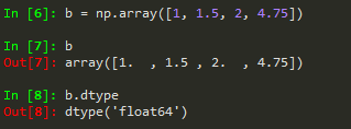
If we pass a list containing values of different types to np.array() NumPy will up-cast the values so they can be of the same type:

The list passed to the array() method contains both integers and floating point numbers. The array created from this list converts the integers to floating point numbers so that all values are of the same type.

**Note: be sure that when you call array() you provide a list of numbers as a single argument :np.array( [1,2,3] ) instead of just the numbers as multiple arguments: np.array( 1,2,3 ) ; this is a pretty common error.

NumPy also allows you to explicitly specify the data type of the array when you create it with the dtype argument:

The values in the array initially are entered as integers, but by specifying the data type as float (dtype = float), Numpy casts all values as floats (ex. 1 → 1.0).

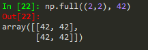
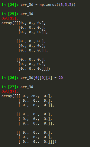
It’s common to know the size of the array, but not know the contents of the array at the time of creation. In this case, NumPy allows the creation of an array of a specified size with placeholder values:

A 3x3 array initialized with all values as 0 with np.zeros( ).

np.ones() and np.empty() can also be used to return an array with all 1’s, or without initializing entries, respectively. If you would like to specify a value to use as a placeholder, use np.full(size, placeholder) :

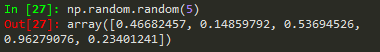
Arrays can also be initialized with random values. Using np.random.random(s) you can create an array of size s filled with random values between 0 and 1. Passing an integer value will yield a 1-D array of that length:

1-D array of length 5.

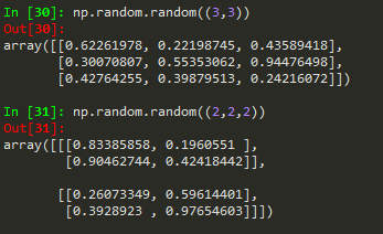
You can pass the dimensions for a higher-dimension array:

Passing (3,3) yields a 2-D 3x3 array, while passing (2,2,2) yields a 3-D 2x2x2 array.

If you want an array with random integer values usenp.random.randint(min, max, size) . Specify the minimum value for min , the maximum value for max , and of course the size of the array for size just as we did with np.random.random() .

In[32]: the range of values is between 0 and 25 for a 2-D 3x3 array. In[33]: the range is between -50 and 50 for a 1-D 10x1 array.

There are a number of other pretty useful ways of creating ndarrays, including:

• filling with evenly-spaced values in a given range
• filling an array with random numbers over a normal distribution
• creating an identity matrix

If you’re interested, check out the array creation documentation to explore these array creation routines along with many others.

---

Array Manipulation

Creating arrays is fine, but where NumPy really shines is the methods for manipulation and computation with arrays. Not only are these methods straightforward and convenient to use, but when it comes to element-wise operations (especially on large arrays), these methods have pretty exceptional performance — much greater than that of iterating through each element, like you might normally do without NumPy.

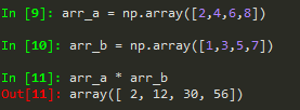
The ndarray object allows us to perform arithmetic operations element-wise on two arrays of the same size:

Each element in b is subtracted from its corresponding element in a. Again, notice all values in the resulting array are floating point, since integers are cast to floats as we saw in the array creation example.

Using the + operator on two ndarrays yields element-wise addition.

Remember, using the + operator between two lists doesn’t add them element-wise. This actually results in concatenation of the two lists. Furthermore, if we try to use the - operator between two lists, Python will return an error since, again, lists do not naturally allow for element-wise operations without explicitly stating so with for-loops.

The statement list_a + list_b concatenates the two lists, while list_a -list_b returns an error.

Element-wise vs Matrix Multiplication

If you have ever used MATLAB before, you know how easy it can be to work with n-dimensional arrays and matrices. NumPy does an excellent job of providing some of that convenient functionality, and may feel much more familiar to MATLAB users than working with bare-bones Python.

Matrix multiplication in MATLAB is as simple as using the * operator on two matrices (e.g. a * b ). With NumPy, the * operator will actually return element-wise multiplication.

For matrix multiplication the @ operator is used for arrays:

---

While on the topic of matrix multiplication, NumPy also has a matrix class, which is actually a subclass of array . The array class is for general purpose use, while the matrix class is intended for linear algebra computations. The documentation recommends that the majority of the time, you should use the array class, unless you are specifically working with linear algebra calculations. If you want to work with higher-dimensional arrays (3-D for example), the array class supports this, while the matrix class is always working with 2 dimensions.

A 3-Dimensional array represented using the ndarray class.

What’s more, the matrix class does not utilize the same operations as array does. So for this article, we will focus on the array class.

---

Just like multiplying two arrays with each other, we can multiply all the elements of an array by a single number. NumPy also makes it really convenient to get properties of arrays, such as the sum, min/max, dimensions of the array ( ndim ), and the size (total elements) of an array.

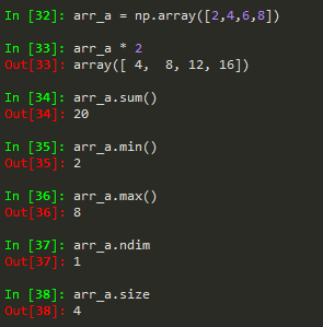
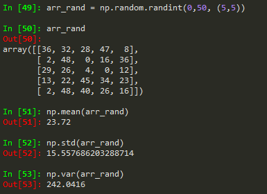
You also have access to basic statistical values for your arrays:

The mean, standard deviation, and variance easily computed for this array.

Get Elements Based on a Condition

One pretty cool numpy class method is numpy.where() . This allows you to return elements from an array that satisfy a specified condition. If, for example, you had a 5x5 array of integers from 0–50, and you wanted to know where the values that are greater than 25 are, you could do the following:

np.where( ) returns a 1 at the indices that hold values greater than 25, and 0 where they are 25 or less. Here r is the original array

If you wanted to find low values (e.g. < 15) and replace them with a -1:

All values less than 15 have been replace with -1. Here arr is the original array in Out[71]

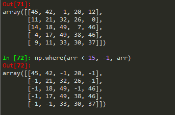
There’s a lot you can do with this method, especially with a little creative thinking, but just remember how it works: np.where(cond[, x, y]) — if cond condition is satisfied, return x , else return y .

Indexing, Slicing, and Reshaping

Indexing works the same as with lists :

Here we create a 3-D array filled with 0’s, then reassign the value at index arr_3d[0][0][1] to 20.

To check if a value is present in an array the in keyword can be used just as with lists :

Slicing works with arrays just as it does with lists , and arrays can be sliced in multiple dimensions:

In[8]: each row in the first 3 columns. In[9]: the first 3 rows in each column. In[10]: all items in the 2nd column.

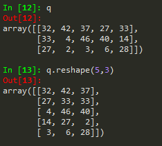
Arrays in NumPy have a lot of functionality when it comes to transformation. For example, if you have a 3x5 array and would like to reshape it to a 5x3:

To reshape an array, pass the desired dimensions to the reshape( ) method.

You can also transpose arrays using array.T:

Array r is the reshape of of the 12x1 array p, to a 3x4 array. Array q is the transpose of r, by using r.T

Arrays can also be transposed using np.transpose(a) , where a is the array you wish to transpose.

---

We’ve really only scratched the surface of what you can do with the NumPy library, and if you’d like to know what else you can do, the official documentation has a great Getting Started guide and, of course, is where you can explore the rest of the library. If you want to use Python for scientific computation, machine learning, or data science, NumPy is one of the libraries that you should really get comfortable with.

Here are a few other related Python libraries I’d recommend checking out, which are considered core in this domain:

• SciPy
• Pandas
• Matplotlib
• Scikit-Learn

To conclude, I’ll send you off with a few resources for continuing your journey in mastering Python for data science and scientific applications.

Python Data Science Handbook by Jake VanderPlas — This is a really excellent primer for getting started with Data Science. He also goes over NumPy towards the beginning, but in much more detail than this article.

Hands-On Machine Learning with Scikit-Learn, Keras & Tensorflow by Aurélien Géron — If you’re really interested in machine learning and deep learning, this book might be the most often recommended book for getting started.

Towards Data Science — Data Science, Machine Learning, AI, general programming. This is one of the best publications on Medium, and is an excellent resource for a huge range of topics relating to Data Science.

Machine Learning Course Offered by Stanford with Andrew Ng — Not exactly specific to Python, but if you’d like to really get into machine learning and dive into some of the theory along with hands-on work, if you have the time to dedicate to the course, this is an excellent place to start. Andrew Ng is brilliant.

Thanks for reading!