A tutorial diving into the gradient descent algorithm for machine learning (ML) with Python
This tutorial’s code is available on Github and its full implementation as well on Google Colab.
Table of Contents
- What is Gradient Descent?
- Cost function
- Gradients
- Python Implementation
- Learning Rate
- Convergence
- Convex Function
- Batch Gradient Descent
- Stochastic Gradient Descent
- Mini-Batch Gradient Descent
- Conclusion
- Resources
- References
📚 Check out our convolutional neural networks tutorial. 📚
What is Gradient Descent?
![Figure 1: A gradient descent illustration | Source: Creative Commons by Wikimedia [3]| Gradient descent algorithm for machine](https://miro.medium.com/max/1100/0*-t2fw32J8jcvZuVm.gif)
Gradient descent is one of the most common machine learning algorithms used in neural networks [7], data science, optimization, and machine learning tasks. The gradient descent algorithm and its variants can be found in almost every machine learning model.
Gradient descent is a popular optimization method of tuning the parameters in a machine learning model. Its goal is to apply optimization to find the least or minimal error value. It is mostly used to update the parameters of the model — in this case, parameters refer to coefficients in regression and weights in a neural network.
A gradient is a vector-valued function that describes the slope of the tangent of a function's graph, pointing to the direction of the most significant rate of increase of the function. It is a derivative that shows the incline or the slope of a cost function [6].
For instance:
Suppose that John is on the top of a mountain, and his goal is to reach the bottom field, but John is blind and cannot see the bottom line. How will he solve this problem?
To solve this problem, he will take small steps around and move towards the higher incline direction, applying these steps iteratively by moving one step at a time until he finally reaches the base of the mountain.
Gradient descent performs in the same way as mentioned in the example. Its primary purpose is to reach the lowest point of the mountain.
![Figure 2: Gradient descent visualization. [2] | Gradient descent algorithm for machine learning (ML) with python tutorial](https://miro.medium.com/max/1400/1*QhPZ4yGFGdXklywNlAk0Wg.png)
It is essential to understand the topics below in detail to understand gradient descent in-depth:
- Cost function
- Minimization of the cost function
- Minima and maxima
- Convex function
- Gradients
- Stopping condition
- Learning rate
Cost Function
Cost function measures the performance of a machine learning algorithm for dispensed data. It quantifies the error within the predicted values and the expected values and impersonates it in the form of a single real number. Fundamentally, it measures the error in prediction perpetrated by an algorithm. It shows the difference between the predicted and the actual values for a given dataset. If the cost function has a lower value, then the model can have a better predictive capability. An excellent value of the cost function is zero — we use the gradient descent algorithm to minimize the cost function.
These are the vital cost functions used in machine learning:
- Mean Squared Error (MSE)
- Log Loss or Cross-Entropy
- KL-Divergence
The equation of Mean Squared Error (MSE):
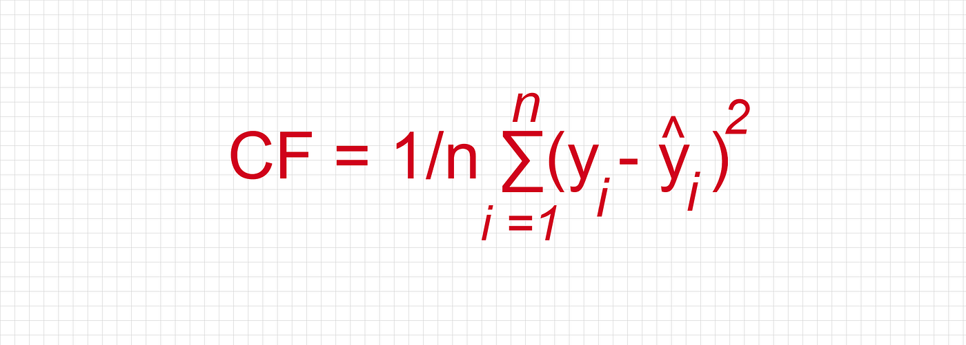
Where:

The mean squared error is used in the regression algorithm in machine learning.
Python code example:
def sum_of_squares(v):
    val = sum(item ** 2 for item in v)
The equation of Log Loss or Cross-Entropy:

The cost function log loss or cross-entropy is used in the classification problem.
Relationship Between Cost Function and Gradient Descent
A cost function is a situation that is minimized. The cost function can be the sum of squared errors over the training set. Gradient descent is a method for finding the minimum of a function of multiple variables [8], and it can be used to minimize the cost function. In summary, If the cost function is a function of K variables, then the gradient is the length-K vector representing the direction in which the cost is growing most quickly.
For instance:
Suppose that there is a case where the regression model will be applied for the binary classification. It is always expected to perform a model with high accuracy and minimal error or loss.
So, in the linear equation → y= mx + c, generally, the parameter values m and c are calculated. Expecting minimal error or loss, such is called the cost function or loss function.
Finding the parameter values m and c with minimal loss is always challenging. In this case, the gradient descent algorithm comes into the picture. Essentially, it helps the model to find the points at which the minimum loss occurs. That is why it has a close relationship with the cost function.
Gradients
The gradient of a straight line shows how steep a straight line is [17].
The equation of the gradient:


A few points related to gradient:
- Up is positive, and down is negative
- Starting from the left and going across to the right is positive.
Let e1, e2, . . . , ed 2 Rd be a specific set of unit vectors so that ei = (0, 0, . . . , 0, 1, 0, . . . , 0) where for ei the 1 is in the ith coordinate.

Gradient descent is a common optimization algorithm used in machine learning to estimate the model parameters. As per calculus, this is a pure partial derivative and gives the input direction in which the function most quickly increases.

Fundamentally, to maximize a function, the algorithm picks a random starting point, measures the gradient, takes a small step in the direction of the gradient, and repeats with the new starting point. Similarly, the function is minimized by taking small steps in the opposite direction. We calculate the cost function based on its initial values, and the parameter estimations are refined over various steps such that the cost function implies a minimum value ultimately.
The gradient descent algorithm:


![Figure 12: Cost function minimization process. [9]. | Gradient descent algorithm for machine learning (ML) with python](https://miro.medium.com/max/1400/0*bFoZqU5P_MnnYpON.png)
The equation of the gradient descent:

Primarily, this formula tells us the next position It needs to go, which is the steepest descent direction.
#Pseudocode
train(θ) = (1/2m) Σ( hθ(x(i)) - y^(i))^2Repeat {
 θj = θj – (learning-rate/m) * Σ( hθ(x^(i)) - y^(i))xj^(i)
    For every j = 0 … n
}
In this case:
xj^(i) is the jth feature of the i^th training example. Next, we repeat until it hits convergence:
- Given the gradient, calculate the changes in the parameters with the learning rate.
- Recalculate the new gradient with the new value of the parameter.
- Repeat step 1.
There are three common types of gradient descent:
- Batch Gradient Descent
- Stochastic Gradient Descent
- Mini-Batch Gradient Descent
Python Implementation of Gradient Descent with Numpy:
Import all required packages:
import pandas as pdimport numpy as npimport matplotlib.pyplot as plt%matplotlib inlineRead data from CSV:
column_names = ['Population', 'Profit']df = pd.read_csv('/content/data.txt', header=None, names=column_names)df.head()
Get the value of X and Y:
df.insert(0, 'Theta0', 1)cols = df.shape[1]X = df.iloc[:,0:cols-1]Y = df.iloc[:,cols-1:cols]theta = np.matrix(np.array([0]*X.shape[1]))X = np.matrix(X.values)Y = np.matrix(Y.values)Plot the data:
df.plot(kind='scatter', x='Population', y='Profit', figsize=(12,8))
Method to calculate RSS:
def calculate_RSS(X, y, theta):
    inner = np.power(((X * theta.T) - y), 2)
    return np.sum(inner) / (2 * len(X))
Method to calculate the gradient descent:
def gradientDescent(X, Y, theta, alpha, iters):
    t = np.matrix(np.zeros(theta.shape))
    parameters = int(theta.ravel().shape[1])
    cost = np.zeros(iters)

    for i in range(iters):
        error = (X * theta.T) - Y    for j in range(parameters):
         term = np.multiply(error, X[:,j])
         t[0,j] = theta[0,j] - ((alpha / len(X)) * np.sum(term))     theta = t
     cost[i] = calculate_RSS(X, Y, theta)     return theta, cost
Calculate error without applying gradient descent:
error = calculate_RSS(X, Y, theta)error
Calculate error by applying gradient descent:
g, cost = gradientDescent(X, Y, theta, 0.01, 1000)g
Calculate error after applying gradient descent:
error = calculate_RSS(X, Y, g)error
Plotting of Data:
x = np.linspace(df.Population.min(), df.Population.max(), 100)f = g[0, 0] + (g[0, 1] * x)fig, ax = plt.subplots(figsize=(12,8))ax.plot(x, f, 'r', label='Prediction')ax.scatter(df.Population, df.Profit, label='Traning Data')ax.legend(loc=2)ax.set_xlabel('Population')ax.set_ylabel('Profit')ax.set_title('Predicted Profit vs. Population Size')
Learning Rate
Learning rate is a hyper-parameter used to control the rate at which an algorithm updates the parameter estimates or learns the parameters' values [9]. It is primarily a tuning parameter in an optimization algorithm and determines the step size at each iteration while moving towards a minimum loss function. It is used to scale the magnitude of parameter updates during gradient descent. It multiplies the gradient by a number (Learning rate or Step size) to determine the next point.
Example:
There is a gradient with a magnitude of 4.2 and a learning rate of 0.01, and then the gradient descent algorithm will pick the next point, 0.042 away from the previous point.
It is essential to understand the local maximum and local minimum concepts to understand the learning rate concept in detail.
Local Maximum
A function f(x) has a local maximum at x = a, and if the value of f(a) is more significant than all the values of f(x) in a small neighborhood of x=a. So, in the mathematical equation shown below:
f(a) > f(a-h) and f(a) > f(a+h). Where, h > 0, then a is called the point of the local maximum.
Fundamentally, a local maximum is a peak position in the landscape that is greater than each of its neighboring states.

Local Minimum
A function f(x) has a local minimum at x = a. If the value of the function at x = a is smaller than the value of the function at the neighboring points of x = a. So, in the mathematical equation shown below:
f (a) < f (a-h) and f (a) < f (a + h). where h > 0, then a is called the point of the local minimum.

Importance of Learning Rate
To reach the local minimum in gradient descent, it is critical to set the learning rate to an appropriate value that is neither too low nor too high. The learning rate is an integral part of it because if the steps it takes are too large, it may not reach the local minimum. After all, it bounces back and forth between the convex function of gradient descent.
If the learning rate is set to a minimal value, then gradient descent will eventually reach the local minimum, however, such may take a while [16].
Two different scenarios can occur in learning rate:
- Big Learning Rate
- Small Learning Rate
Thus, the learning rate should never be too high or too low per the different scenarios shown above. If the learning rate is too large, the oscillation will diverge.
Showing the learning rate:
def step_gradient(b_current, m_current, points, learning_rate):
    b_gradient = 0
    m_gradient = 0
    n = float(len(points))

    for i in range(0, len(points)):
        x = points[i, 0]
        y = points[i, 1]
        b_gradient += -(2/n) * (y - ((m_current * x) + b_current))
        m_gradient += -(2/n) * x * (y - ((m_current * x) + b_current))

    latest_b = b_current - (learning_rate * b_gradient)
    latest_m = m_current - (learning_rate * m_gradient)
    return [latest_b, latest_m]
Convergence
Convergence is a name given to the position where the loss function does not improve significantly, and we are stuck at a point near the minima. If the cost function should decrease after every iteration, then it is said that gradient descent is working correctly. If the gradient descent does not decrease the cost-function anymore and remains more or less on the same level, it converges.
Gradient descent converges to a local minimum when it begins close enough to that minimum. If there are multiple local minimums, its convergence depends on the point where the iteration starts. It is challenging to converge to a global minimum.
Convergence always depends on the type of function on which optimization is used. If the objective function is convex, the gradient descent always converges to the same local minima, and it is also the global minimum.

Convex Function
If the line segment between any two points on the graph of the function lies above or on the graph [15], it is a convex function.
Mathematically, the convex function can be defined as:
A convex function is a function whose value at the midpoint of every interval in its domain does not exceed the arithmetic mean of its values at the ends of the interval [14].

Thus diving into the mathematical equation:
There is an interval [a, b] and f(x) is a function and x1 and x2 are two points in the interval [a, b] and any λ where 0 < λ < 1. So,

![Figure 26: Convex function on the interval | Source: Wikipedia [5], License CC BY-SA 3.0](https://miro.medium.com/max/1400/0*iupLPYz1HHYGqxm1.png)
Primary Types of Gradient Descent
Batch Gradient Descent (BGD)
Batch gradient descent calculates the error for each example in the training dataset but only updates the model after all training examples have been evaluated [13]. It is excellent for convex or relatively smooth error manifolds. It is computationally costly, but it scales well with the number of features. The following are crucial for batch gradient descent:
- It is very slow and computationally expensive.
- It is never suggested to use the vast training dataset.
- Here, convergence is slow.
- It computes the gradient using the whole training dataset.
Stochastic Gradient Descent (SGD)
There is a situation in batch gradient descent mentioned below:
Imagine that there is a dataset with 5 million examples. So, to take one step, the model will calculate the gradients of all 5 million examples. This type of situation happens in the batch gradient descent.
The above situation is inefficient, so stochastic gradient descent is in the picture to handle this problem. Essentially, it calculates the error and updates the model for each example in the training dataset.
Stochastic gradient descent has the following points:
- It computes gradient using a single training sample.
- It is suggested to use with large training samples.
- It is faster and less computationally expensive in comparison with Batch Gradient Descent.
- It reaches the convergence much faster.
- It can shallow local minima more easily.
Mini-batch Gradient Descent (MBGD)
Mini-batch gradient descent splits the training dataset into small batches, and these batches are used to calculate model error and update model coefficients. It can be used for smoother curves.
The mini-batch gradient descent has the following essential points:
- It can be used when the dataset is large.
- It converges directly to minima.
- It is faster to larger datasets.
- Since in SGD, only one example is used simultaneously, so vectorized implementation cannot be implemented.
- It can slow down the computations — to stop this problem, a mixture of batch gradient descent and SGD is used.

Conclusion
Gradient descent is a first-order iterative optimization algorithm [10] for obtaining a local minimum of a differentiable function. It bases on a convex function and tweaks its parameters iteratively to minimize a given function to its local minimum.
In terms of types of gradient descent, batch gradient descent (BGD) is the most common form of gradient descent used in machine learning [12]. Some day-to-day algorithms with coefficients that can be optimized using gradient descent methods are Linear Regression and Logistic Regression [11].
The loss function explains how great the model will perform presented the current set of parameters (weights and biases), and gradient descent is used to find the best set of parameters.
DISCLAIMER: The views expressed in this article are those of the author(s) and do not represent the views of Carnegie Mellon University nor other companies (directly or indirectly) associated with the author(s). These writings do not intend to be final products, yet rather a reflection of current thinking, along with being a catalyst for discussion and improvement.
All images are from the author(s) unless stated otherwise.
Published via Towards AI
Resources
References
[1] MATLAB mesh sic3D.svg, Wikimedia Commons, https://commons.wikimedia.org/wiki/File:MATLAB_mesh_sinc3D.svg
[2] 從 Gradient Descent to Optimizer, by ITHome, https://ithelp.ithome.com.tw/articles/10218912
[3] Gradient descent, Wikimedia Commons, https://commons.wikimedia.org/wiki/File:Gradient_descent.gif
[4] Local and Global Maxima and Minima, Wikipedia, License GFDL 1.2, https://en.wikipedia.org/wiki/Maxima_and_minima#/media/File:Extrema_example_original.svg
[5] Convex Function on An Interval, Wikipedia, License CC BY-SA 3.0, https://en.wikipedia.org/wiki/Convex_function#/media/File:ConvexFunction.svg
[6] The Gradient and Directional Derivative, Oregon State University, http://sites.science.oregonstate.edu/math/home/programs/undergrad/CalculusQuestStudyGuides/vcalc/grad/grad.html
[7] Gemulla, Rainer & Nijkamp, Erik & Haas, Peter & Sismanis, Yannis. (2011). Large-scale matrix factorization with distributed stochastic gradient descent. Proceedings of the ACM SIGKDD International Conference on Knowledge Discovery and Data Mining. 69–77. 10.1145/2020408.2020426.
[8] Minimizing the cost function: Gradient descent, XuanKhanh Nguyen, Towards Data Science, https://towardsdatascience.com/minimizing-the-cost-function-gradient-descent-a5dd6b5350e1
[9] Understanding Learning Rate in Machine Learning, Great Learning Team, https://www.mygreatlearning.com/blog/understanding-learning-rate-in-machine-learning/
[10] Gradient Descent, Wikipedia, https://en.wikipedia.org/wiki/Gradient_descent
[11] Gradient Descent for Machine Learning, Machine Learning Mastery, https://machinelearningmastery.com/gradient-descent-for-machine-learning/
[12] Master Machine Learning Algorithms, Jason Brownlee, Ph.D., https://machinelearningmastery.com/master-machine-learning-algorithms/
[13] A Gentle Introduction to Mini-batch Gradient Descent and How to Configure Batch Size, Machine Learning Mastery, https://machinelearningmastery.com/gentle-introduction-mini-batch-gradient-descent-configure-batch-size/
[14] Convex Function, The Art of Problem Solving, https://artofproblemsolving.com/wiki/index.php/Convex_function
[15] Gradient Descent Unraveled, Manpreet Singh Minhas, https://towardsdatascience.com/gradient-descent-unraveled-3274c895d12d
[16] Gradient Descent: An Introduction to 1 of Machine Learning’s Most Popular Algorithms, Niklas Donges, https://builtin.com/data-science/gradient-descent
[17] Gradient (Slope) of Straight Line, Math is Fun, https://www.mathsisfun.com/gradient.html


No comments:
Post a Comment