This series of articles was designed to explain how to use Python in a simplistic way to fuel your company’s growth by applying the predictive approach to all your actions. It will be a combination of programming, data analysis, and machine learning.
I will cover all the topics in the following nine articles:
Articles will have their own code snippets to make you easily apply them. If you are super new to programming, you can have a good introduction forPythonandPandas(a famous library that we will use on everything) here. But still without a coding introduction, you can learn the concepts, how to use your data and start generating value out of it:
Sometimes you gotta run before you can walk — Tony Stark
As a pre-requisite, be sure Jupyter Notebookand Pythonare installed on your computer. The code snippets will run on Jupyter Notebook only.
Alright, let’s start.
Part 5: Predicting Next Purchase Day
Most of the actions we explained in Data Driven Growth series have the same mentality behind:
Treat your customers in a way they deserve before they expect that (e.g., LTV prediction) and act before something bad happens (e.g., churn).
Predictive analytics helps us a lot on this one. One of the many opportunities it can provide is predicting the next purchase day of the customer. What if you know if a customer is likely to make another purchase in 7 days?
We can build our strategy on top of that and come up with lots of tactical actions like:
No promotional offer to this customer since s/he will make a purchase anyways
Nudge the customer with inbound marketing if there is no purchase in the predicted time window (or fire the guy who did the prediction 🦹♀️ 🦹♂️ )
Data Wrangling (creating previous/next datasets and calculate purchase day differences)
Feature Engineering
Selecting a Machine Learning Model
Multi-Classification Model
Hyperparameter Tuning
Data Wrangling
Let’s start with importing our data and do the preliminary data work:
Importing CSV file and date field transformation
We have imported the CSV file, converted the date field from string to DateTime to make it workable and filtered out countries other than the UK.
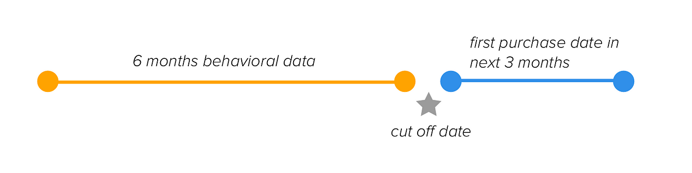
To build our model, we should split our data into two parts:
Data structure for training the model
We use six months of behavioral data to predict customers’ first purchase date in the next three months. If there is no purchase, we will predict that too. Let’s assume our cut off date is Sep 9th ’11 and split the data:
tx_6mrepresents the six months performance whereas we will usetx_nextfor the find out the days between the last purchase date in tx_6m and the first one in tx_next.
Also, we will create a dataframe calledtx_userto possess a user-level feature set for the prediction model:
By using the data in tx_next, we need the calculate ourlabel(days between last purchase before cut off date and first purchase after that):
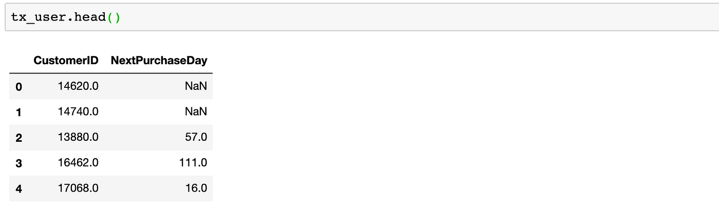
Now, tx_user looks like below:
As you can easily notice, we have NaN values because those customers haven’t made any purchase yet. We fill NaN with 999 to quickly identify them later.
We have customer ids and corresponding labels in a dataframe. Let’s enrich it with our feature set to build our machine learning model.
Feature Engineering
For this project, we have selected our feature candidates like below:
RFM scores & clusters
Days between the last three purchases
Mean & standard deviation of the difference between purchases in days
After adding these features, we need to deal with the categorical features by applyingget_dummiesmethod.
For RFM, to not repeatPart 2, we share the code block and move forward:
RFM Scores & Clustering
Let’s focus on how we can add the next two features. We will be usingshift()method a lot in this part.
First, we create a dataframe with Customer ID and Invoice Day (not datetime). Then we will remove the duplicates since customers can do multiple purchases in a day and difference will become 0 for those.
#create a dataframe with CustomerID and Invoice Date
tx_day_order = tx_6m[['CustomerID','InvoiceDate']]#convert Invoice Datetime to day
tx_day_order['InvoiceDay'] = tx_6m['InvoiceDate'].dt.datetx_day_order = tx_day_order.sort_values(['CustomerID','InvoiceDate'])#drop duplicates
tx_day_order = tx_day_order.drop_duplicates(subset=['CustomerID','InvoiceDay'],keep='first')
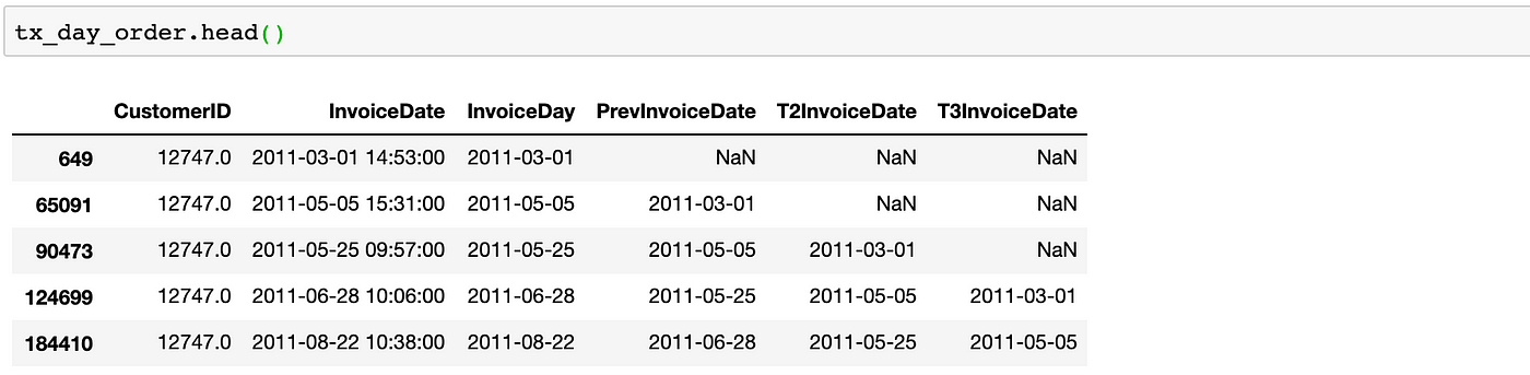
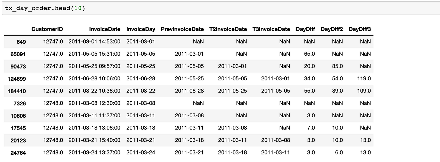
Next, by using shift, we create new columns with the dates of last 3 purchases and see how our dataframe looks like:
Now we are going to make a tough decision. The calculation above is quite useful for customers who have many purchases. But we can’t say the same for the ones with 1–2 purchases. For instance, it is too early to tag a customer asfrequentwho has only 2 purchases but back to back.
We only keep customers who have > 3 purchases by using the following line:
Finally, we drop NA values, merge new dataframes with tx_user and apply.get_dummies()forconverting categorical values:
tx_day_order_last = tx_day_order_last.dropna()tx_day_order_last = pd.merge(tx_day_order_last, tx_day_diff, on='CustomerID')tx_user = pd.merge(tx_user, tx_day_order_last[['CustomerID','DayDiff','DayDiff2','DayDiff3','DayDiffMean','DayDiffStd']], on='CustomerID')#create tx_class as a copy of tx_user before applying get_dummies
tx_class = tx_user.copy()
tx_class = pd.get_dummies(tx_class)
Our feature set is ready for building a classification model. But there are many different models, which one should we use?
Selecting a Machine Learning Model
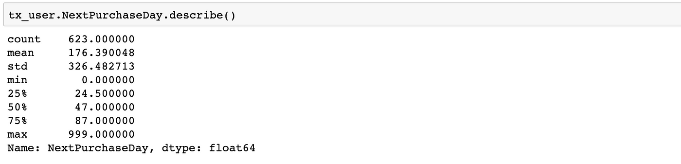
Before jumping into choosing the model, we need to take two actions. First, we need to identify the classes in our label. Generally, percentiles give the right for that. Let’s use.describe()method to see them inNextPurchaseDay:
Deciding the boundaries is a question for both statistics and business needs. It should make sense in terms of the first one and be easy to take action and communicate. Considering these two, we will have three classes:
0–20: Customers that will purchase in 0–20 days —Class name: 2
21–49: Customers that will purchase in 21–49 days —Class name: 1
≥ 50: Customers that will purchase in more than 50 days —Class name: 0
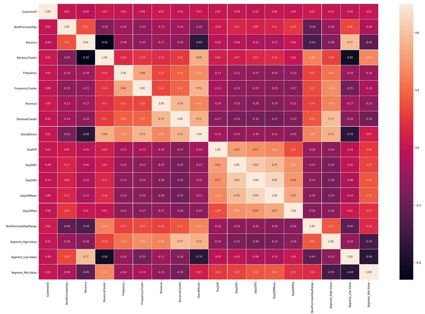
Looks likeOverall Scorehas the highest positive correlation (0.45) andRecencyhas the highest negative (-0.54).
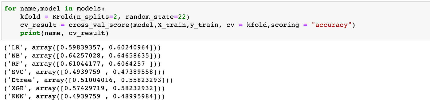
For this particular problem, we want to use the model which gives the highest accuracy. Let’s split train and test tests and measure the accuracy of different models:
Selecting the ML model for the best accuracy
Accuracy per each model:
From this result, we see that Naive Bayes is the best performing one (~64% accuracy). But before that, let’s look at what we did exactly. We applied a fundamental concept in Machine Learning, which isCross Validation.
How can we be sure of the stability of our machine learning model across different datasets? Also, what if there is a noise in the test set we selected.
Cross Validation is a way of measuring this. It provides the score of the model by selecting different test sets. If the deviation is low, it means the model is stable. In our case, the deviations between scores are acceptable (except Decision Tree Classifier).
Normally, we should go ahead with Naive Bayes. But for this example, let’s move forward with XGBoost to show how we can improve an existing model with some advanced techniques.
Multi-Classification Model
To build our model, we will follow the steps in the previous articles. But for improving it further, we’ll do Hyperparameter Tuning.
Programmatically, we will find out what are the best parameters for our model to make it provide the best accuracy.
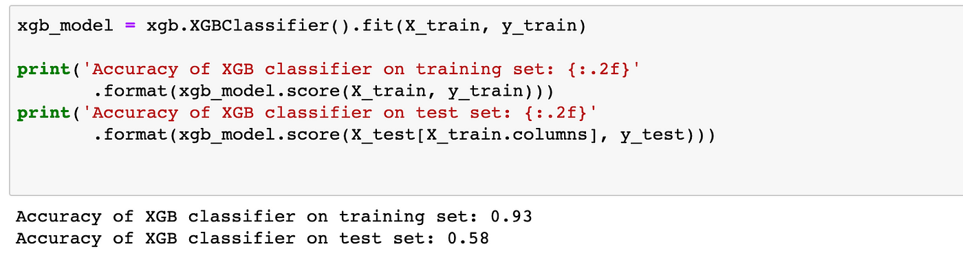
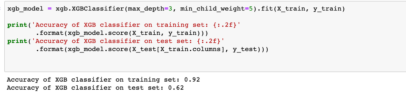
Let’s start with coding our model first:
xgb_model = xgb.XGBClassifier().fit(X_train, y_train)print('Accuracy of XGB classifier on training set: {:.2f}'
       .format(xgb_model.score(X_train, y_train)))
print('Accuracy of XGB classifier on test set: {:.2f}'
       .format(xgb_model.score(X_test[X_train.columns], y_test)))
In this version, our accuracy on the test set is 58%:
XGBClassifier has many parameters. You can find the list of them here. For this example, we will select max_depth and min_child_weight.
The code below will generate the best values for these parameters:
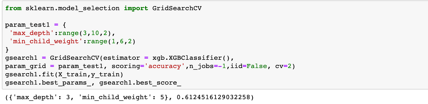


No comments:
Post a Comment