Saturday, April 18, 2020

How to train a neural network on Chrome using tensorflow.js

This tutorial is just a demonstration of how we can make use of simple scripting languages (like javascript). In this case, to train and predict using a neural network in the browser. We are going to use javascript. The main objective of this blog is to make use of a browser not only for using the internet but also for training a model behind the scenes.
In this tutorial, we’re going to build a model that infers the relationship between two numbers where y = 2x -1 (y equals 2x minus 1).
So let’s begin with our tutorial.

Things we need for this tutorial
1. A simple HTML file containing a .js snippet.
2. A Google Chrome Browser.
3. A text editor to edit html file.

Let’s start with creating a basic html file

<!DOCTYPE html>
<html>
<head>
 <title>Training a model on browser</title>
</head>
<body></body>
</html>

Now we need to import tensorflow.js library

<script src="https://cdn.jsdelivr.net/npm/@tensorflow/tfjs@latest"></script>
Note: this must be included inside <head> tag

Creating a function for training

function doTraining(model) {
//here we are going to write logic for training
}
We need to make function asynchronous so that it can run in the background without affecting our webpage.
async function doTraining(model){
            const history = 
                  await model.fit(xs, ys, 
                        { epochs: 500,
                          callbacks:{
                              onEpochEnd: async(epoch, logs) =>{
                                  console.log("Epoch:" 
                                              + epoch 
                                              + " Loss:" 
                                              + logs.loss);
                                  
                              }
                          }
                        });
        }
Function Explanation:
We are calling model.fit() asynchronously inside our function, in order to do that we need to pass the model as a parameter to our async function.
We have used await with the model so that it can wait until the training finished. It won’t affect our web page because of async call.
We have used javascript callbacks for after training purposes like in this case we have called onEpochEnd to print the final loss after the training completes.
Now that we are ready with our function we can proceed with prediction.

Creating a model with single neural network

const model = tf.sequential();model.add(tf.layers.dense({units: 1, inputShape: [1]}));model.compile({loss:'meanSquaredError', 
                       optimizer:'sgd'});

Model Summary

model.summary()
//pretty simple
A model summary with 1 neuron network
P.S.: Those who are thinking why did the summary display Trainable params: 2 (two)
There are two params because of 
Weights and Biases i.e w and c

Sample numeric data for training our equation

const xs = tf.tensor2d([-1.0, 0.0, 1.0, 2.0, 3.0, 4.0], [6, 1]);const ys = tf.tensor2d([-3.0, -1.0, 2.0, 3.0, 5.0, 7.0], [6, 1]);
Explanation:
Just like we use numpy in python , we need to use tf.tensor2d() function for defining a two-dimensional array.
It’s important to mention shape of array to the tensor2d function.
let xs = [-1.0, 0.0, 1.0, 2.0, 3.0, 4.0] # array[6,1] # shape of that array

Asynchronously training and predicting

doTraining(model).then(() => {
            alert(model.predict(tf.tensor2d([10], [1,1])));
        }); #calling the function
We are going to use Promise.js for asynchronously calling the training function and then predicting a value based on the trained model.
Those who are new to javascript can check what is Promise.js from here.

Adding some data to show on webpage.

<h1 align="center">Press 'f12' key or 'Ctrl' + 'Shift' + 'i' to check whats going on</h1>
We can also add some data that will be displayed on web page just like a sample running website.

The final html file will look like this

<!DOCTYPE html>
<html>
<head>
 <title>Training a model on browser</title>
 <script src="https://cdn.jsdelivr.net/npm/@tensorflow/tfjs@latest"></script><script lang="js">
        async function doTraining(model){
            const history = 
                  await model.fit(xs, ys, 
                        { epochs: 500,
                          callbacks:{
                              onEpochEnd: async(epoch, logs) =>{
                                  console.log("Epoch:" 
                                              + epoch 
                                              + " Loss:" 
                                              + logs.loss);
                                  
                              }
                          }
                        });
        }
        const model = tf.sequential();
        model.add(tf.layers.dense({units: 1, inputShape: [1]}));
        model.compile({loss:'meanSquaredError', 
                       optimizer:'sgd'});
        model.summary();
   const xs = tf.tensor2d([-1.0, 0.0, 1.0, 2.0, 3.0, 4.0], [6, 1]);
   const ys = tf.tensor2d([-3.0, -1.0, 2.0, 3.0, 5.0, 7.0], [6, 1]);
        doTraining(model).then(() => {
            alert(model.predict(tf.tensor2d([10], [1,1])));
        });
    </script>
</head>
<body>
 <h1 align="center">Press 'f12' key or 'Ctrl' + 'Shift' + 'i' to check whats going on</h1>
</body>
</html>
You can also download this file from here.

Finally training and predicting your model on browser

Open your html file with Google Chrome and check the developer console by pressing ‘F12’ key.
A snapshot of training log in console followed by prediction in alert box
A snapshot of training log in console followed by prediction in the alert box
You can see the training epochs with their loss inside the developer console. An alert box will be automatically displayed on a webpage with prediction results as soon as the training completes.
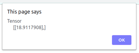
An image containing prediction for the input 10 for equation y = 2x-1
This is an alert box displaying the prediction for our input number which is 10.
According to the equation Y = 2X-1 the output for input x = 10 should be
y = 19. Our model predicted 18.91 which is close enough.

Thank You

Please feel free to share your doubts or suggestions. I am one of the members of team Nsemble.ai, we love to research and develop challenging products using artificial intelligence. Nsemble have developed several solution in the domain of Industry 4.0 and E-commerce. We will be happy to help you.

Monday, April 13, 2020

Beginner’s Guide to Data Science Libraries in Python


NumPy

This is the most fundamental library that all data scientists need to learn. It provides all of the basic functions in scientific computing and is able to process lots of data quickly. The following code is a quick example of what NumPy can do.
Sample of using NumPy for scientific calculations
Input:  [0, 1.5707963267948966, 3.141592653589793, 4.71238898038469, 6.283185307179586]Sine values:  [ 0.0000000e+00  1.0000000e+00  1.2246468e-16 -1.0000000e+00-2.4492936e-16]Cosine values:  [ 1.0000000e+00  6.1232340e-17 -1.0000000e+00 -1.8369702e-161.0000000e+00]Sine values:  [ 0.  1.  0. -1. -0.]Cosine values:  [ 1.  0. -1. -0.  1.]

pandas

This is the most fundamental library for data analysis and manipulation in Python. This library is able to quickly read large raw data files into a DataFrame object, perform all kinds of data cleaning and data mining operations with automatic indexing and data alignment, execute all possible SQL queries on the DataFrame table, such as joins and merges, and then output the data into another data file or even directly into visualizations.
df = pd.DataFrame('some data...')df.plot(x='label1', y='label2', kind='scatter', ...)
Sample scatterplot of Area vs. Population [source]

SciPy

The SciPy library is an abstracted layer on top of NumPy and the rest of the SciPy stack. This library includes many numerical routines such as numerical integration, interpolation, optimization, linear algebra, statistics, special functions, FFT, signal and image processing, ODE solvers and other tasks common in science and engineering. Therefore, this library is more specific to mathematical functions that tailor towards calculations done by scientists and engineers from an academic standpoint. To learn more, visit the official documentation site.

Scikit-Learn

The Scikit-Learn library is further abstracted on top of SciPy and is more practical and application focused. This library includes functions that focuses more on machine learning applications such as regression, classification, clustering, etc. People who are passionate about machine learning will definitely want to learn more about functionalities that this library provides. For example, you can easily run a RANSAC linear regression on a set of raw data by running the following code:
# generate random data with a small set of outliers
np.random.seed(0)
X[:n_outliers] = 3 + 0.5 * np.random.normal(size=(n_outliers, 1))
y[:n_outliers] = -3 + 10 * np.random.normal(size=n_outliers)

# Fit line using all data
lr = linear_model.LinearRegression()
lr.fit(X, y)

# Robustly fit linear model with RANSAC algorithm
ransac = linear_model.RANSACRegressor()
ransac.fit(X, y)
inlier_mask = ransac.inlier_mask_
outlier_mask = np.logical_not(inlier_mask)

# Predict data of estimated models
line_X = np.arange(X.min(), X.max())[:, np.newaxis]
line_y = lr.predict(line_X)
line_y_ransac = ransac.predict(line_X)
Scatterplot of Raw data and Linear Regression vs. RANSAC Regression of data [source]
sklearn.model_selection.train_test_split(*arrays, **options)[source]

matplotlib.pyplot

This library, although has nothing to do with the analytics portion of data science, is also a key library to learn and use. This library is the Python adaptation of Matlab’s plotting functionality. This library is able to generate anything from simple scatterplots, histograms, line plots to complex heatmaps, 3D plots, eclipses, streamplots, etc. Some examples of these plots are below:
Sample scatterplot with color-coding [source]
Sample 3D plot [source]
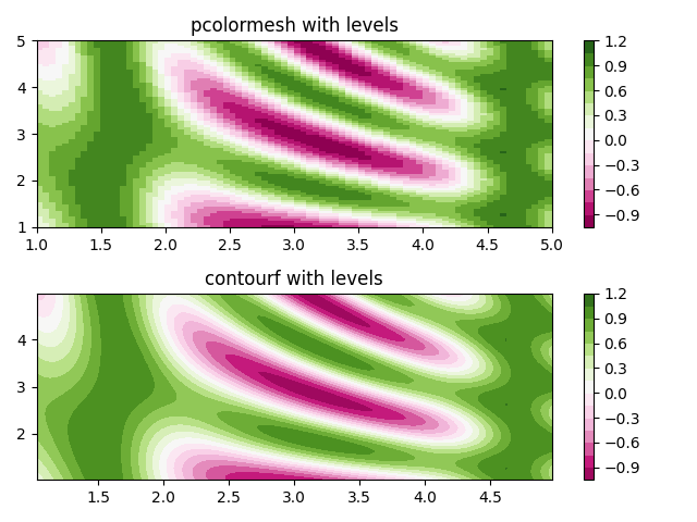
Sample visualization of 2D array [source]

Conclusion

There are lots of Python libraries that I did not cover. There are lots of libraries targeted towards bio-informatics, deep-learning and AI, self-driving, etc. However, the libraries outlined here are widely used in data science and are the building blocks of many advanced Python libraries. I believe that becoming familiar with these libraries will build up a strong foundation for a beginner who wants to explore the field of data science. If there are any other common Python libraries that you think would be useful to learn, please share them in the comments below.

Saturday, April 11, 2020

Numpy Array Cookbook: Generating and Manipulating Arrays in Python


1) Array Overview

What are Arrays?

Array’s are a data structure for storing homogeneous data. That mean’s all elements are the same type.
import numpy as nparr = np.array([[1,2],[3,4]])
type(arr)#=> numpy.ndarray
np.zeros((2))
#=> array([0., 0.])np.zeros((2,2))
#=> array([[0., 0.],
#=>        [0., 0.]])np.zeros((2,2,2))
#=> array([[[0., 0.],
#=>         [0., 0.]],
#=> 
#=>        [[0., 0.],
#=>         [0., 0.]]])
...

Arrays vs Lists

  • Arrays use less memory than lists
  • Arrays have significantly more functionality
  • Arrays require data to be homogeneous; lists do not
  • Arithmetic on arrays operates like matrix multiplication

Important Parameters

shape: a tuple representing dimensions of an array. An array of shape (2,3,2) is a 2x3x2 dimension array. And looks like below.
np.zeros((2,3,2))#=> array([[[0., 0.],
#=>         [0., 0.],
#=>         [0., 0.]],
#=> 
#=>        [[0., 0.],
#=>         [0., 0.],
#=>         [0., 0.]]])

2) Generating Arrays

zeros

Generate an array of zeros with a specified shape.
np.zeros((2,3))
#=> array([[0., 0., 0.],
#=>        [0., 0., 0.]])

ones

Generate an array of ones with a specified shape.
np.ones((2,3))
#=> array([[1., 1., 1.],
#=>        [1., 1., 1.]])

empty

np.empty() is a little different than zeros and ones, as it doesn’t preset any values in the array. Some people say it’s slightly faster to initialize but that’s negligible.
arr = np.empty((2,2))
arr
#=> array([[1.00000000e+000, 1.49166815e-154],
#=>        [4.44659081e-323, 0.00000000e+000]])

full

Initialize an array with a given value.
np.full((3,2), 10)
#=> array([[10, 10],
#=>        [10, 10],
#=>        [10, 10]])np.full((3,2), ['a','b'])
#=> array([['a', 'b'],
#=>        ['a', 'b'],
#=>        ['a', 'b']], dtype='<U1')

array

This is probably what you’ve seen the most in real life. It initializes an array from an “array-like” object.
li = ['a','b','c']
np.array(li)#=> array(['a', 'b', 'c'], dtype='<U1')

_like

There are several _like functions corresponding to the functions we’ve discussed: empty_likeones_likezeros_like and full_like.
a1 = np.array([[1,2],[3,4]])
#=> array([[1, 2],
#=>        [3, 4]])np.ones_like(a1)
#=> array([[1, 1],
#=>        [1, 1]])

rand

Generate an array with random values.
np.random.rand(3,2)
#=> array([[0.94664048, 0.76616114],
#=>        [0.395549  , 0.84680126],
#=>        [0.42873   , 0.77736086]])

asarray

np.asarray is a wrapper around np.array, which sets the parameter copy=False. See np.array above.

arange

Generates an array of values with a set interval between an upper and lower limit. It’s numpy’s version of list(range(50,60,2)) with lists.
np.arange(50,60,2)
#=> array([50, 52, 54, 56, 58])

linspace

Generates an array of numbers with equal intervals between 2 other numbers. Instead of specifying the interval directly like arange, we specify how many numbers to generate between the upper and lower limit.
np.linspace(10, 20, 6)
#=> array([10., 12., 14., 16., 18., 20.])np.linspace(0, 2, 5)
#=> array([0. , 0.5, 1. , 1.5, 2. ])

meshgrid

Generates a matrix of coordinates based on 2 input arrays.
x = np.array([1,2,3])
y = np.array([-3,-2,-1])
 
xcors, ycors = np.meshgrid(x, y) xcors
#=> [[1 2 3]
#=> [1 2 3]
#=> [1 2 3]]ycors
#=> [[-3 -3 -3]
#=> [-2 -2 -2]
#=> [-1 -1 -1]]
[[(1, -3), (2, -3), (3, -3)]
 [(1, -2), (2, -2), (3, -2)],
 [(1, -1), (2, -1), (3, -1)]]

3) Manipulating Arrays

copy

Make a copy of an existing array.
a1 = np.array([1,2,3])
a2 = a1a2[0] = 10
a1
#=> array([10,  2,  3])
a1 = np.array([1,2,3])
a2 = a1.copy()a2[0] = 10
a1
#=> array([1, 2, 3])

shape

Get the shape of an array.
a = np.array([[1,2],[3,4],[5,6]])
a.shape
#=> (3, 2)

reshape

Reshapes an array.
a = np.array([[1,2],[3,4],[5,6]])
a
#=> array([[1, 2],
#=>        [3, 4],
#=>        [5, 6]])
a.shape
#=> (3, 2)
a.reshape(2,3)
#=> array([[1, 2, 3],
#=>        [4, 5, 6]])
a.reshape(6)
#=> array([1, 2, 3, 4, 5, 6])
a.reshape(6,1)
#=>array([[1],
#=>       [2],
#=>       [3],
#=>       [4],
#=>       [5],
#=>       [6]])
a.reshape(2,3,1)
#=> array([[[1],
#=>         [2],
#=>         [3]],
#=> 
#=>        [[4],
#=>         [5],
#=>         [6]]])

resize

Similar to reshape but it mutates the original array.
a = np.array([['a','b'],['c','d']])
a
#=>array([['a', 'b'],
#=>       ['c', 'd']], dtype='<U1')a.reshape(1,4)
#=> array([['a', 'b', 'c', 'd']], dtype='<U1')a
#=>array([['a', 'b'],
#=>       ['c', 'd']], dtype='<U1')a.resize(1,4)
a
#=> array([['a', 'b', 'c', 'd']], dtype='<U1')

transpose

Transposes an array.
a = np.array([['s','t','u'],['x','y','z']])
a
#=> array([['s', 't', 'u'],
#=>        ['x', 'y', 'z']], dtype='<U1')a.T
#=> array([['s', 'x'],
#=>        ['t', 'y'],
#=>        ['u', 'z']], dtype='<U1')

flatten

Flattens an array into 1 dimension and returns a copy.
a = np.array([[1,2,3],['a','b','c']])
a.flatten()
#=> array(['1', '2', '3', 'a', 'b', 'c'], dtype='<U21')a.reshape(6)
#=> array(['1', '2', '3', 'a', 'b', 'c'], dtype='<U21')

ravel

Flattens an array-like object into 1 dimension. Similar to flatten but it returns a view of an array instead of a copy.
np.ravel([[1,2,3],[4,5,6]])
#=> array([1, 2, 3, 4, 5, 6])np.flatten([[1,2,3],[4,5,6]])
#=> AttributeError: module 'numpy' has no attribute 'flatten'

hsplit

Horizontally splits an array into subarrays.
a = np.array(
    [[1,2,3],
     [4,5,6]])
a
#=> array([[1, 2, 3],
#=>        [4, 5, 6]])np.hsplit(a,3)# #=> [array([[1],[4]]), 
# #=>  array([[2],[5]]), 
# #=>  array([[3],[6]])]

vsplit

Vertically splits an array into subarrays.
a = np.array(
    [[1,2,3],
     [4,5,6]])
a
#=> array([[1, 2, 3],
#=>        [4, 5, 6]])np.vsplit(a,2)#=> [array([[1, 2, 3]]), 
#=> array([[4, 5, 6]])]

stack

Joins arrays on an axis.
a = np.array(['a', 'b', 'c'])
b = np.array(['d', 'e', 'f'])np.stack((a, b), axis=0)
#=> array([['a', 'b', 'c'],
#=>       ['d', 'e', 'f']], dtype='<U1')
a = np.array(['a', 'b', 'c'])
b = np.array(['d', 'e', 'f'])np.stack((a, b), axis=1)
#=> array([['a', 'd'],
#=>        ['b', 'e'],
#=>        ['c', 'f']], dtype='<U1')

Conclusion

I consider this the basics of numpy. You’ll come across these functions repeatedly when reading existing code at work or doing tutorials online.

Must Watch YouTube Videos for Databricks Platform Administrators

  While written word is clearly the medium of choice for this platform, sometimes a picture or a video can be worth 1,000 words. Below are  ...