Saturday, February 24, 2024

7 Vector Databases Every AI/ML/Data Engineer Should Know!


In the rapidly evolving fields of artificial intelligence (AI), machine learning (ML), and data engineering, the need for efficient data storage and retrieval systems is paramount. Vector databases have emerged as a critical solution for managing the complex, high-dimensional data that these technologies often rely on. Here, we explore seven vector databases that every AI/ML/data engineer should be familiar with, highlighting their unique features and how they support the demands of modern data-driven applications.

1. Milvus

Milvus is an open-source vector database designed to handle large-scale similarity search and vector indexing. It supports multiple index types and offers highly efficient search capabilities, making it suitable for a wide range of AI and ML applications, including image and video recognition, natural language processing, and recommendation systems.

Key Features:

  • Highly scalable, supporting billions of vectors.
  • Supports multiple metric types for similarity search.
  • Easy integration with popular machine learning frameworks.
  • Robust and flexible indexing mechanisms.

Try Milvus!

2. Pinecone

Pinecone is a managed vector database service that simplifies the process of building and scaling vector search applications. It offers a simple API for embedding vector search into applications, providing accurate, scalable similarity search with minimal setup and maintenance.

Key Features:

  • Managed service with easy setup and scalability.
  • Accurate similarity search with sub-second latencies.
  • Supports updates and deletions in real-time.
  • Integrates easily with existing data pipelines and ML models.

Try Pinecone!

3. SingleStore Database

SingleStore Database started supporting vector storage as a feature back in 2017 when vector databases were not even a thing.

The robust vector database capabilities of SingleStoreDB are tailored to seamlessly serve AI-driven applications, chatbots, image recognition systems and more. With SingleStoreDB, the necessity for maintaining a dedicated vector database for your vector-intensive workloads becomes obsolete.

Diverging from conventional vector database approaches, SingleStoreDB takes a novel approach by housing vector data within relational tables alongside diverse data types. This innovative amalgamation empowers you to effortlessly access comprehensive metadata and additional attributes pertaining to your vector data, all while leveraging the extensive querying prowess of SQL.

SingleStore’s latest new features for vector search

We are thrilled to announce the arrival of SingleStore Pro Max One of the highlights of the release includes vector search enhancements.

Two important new features have been added to improve vector data processing, and the performance of vector search.

  1. Indexed approximate-nearest-neighbor (ANN) search
  2. A VECTOR data type

Indexed ANN vector search facilitates creation of large-scale semantic search and generative AI applications. Supported index types include inverted file (IVF), hierarchical navigable small world (HNSW) and variants of both based on product quantization (PQ) — a vector compression method. The VECTOR type makes it easier to create, test, and debug vector-based applications. New infix operators are available for DOT_PRODUCT (<*>) and EUCLIDEAN_DISTANCE (<->) to help shorten queries and make them more readable.

Key Features:

  • Real-time analytics and HTAP capabilities for GenAI applications.
  • Highly scalable vector store support.
  • Scalable, distributed architecture.
  • Support for SQL and JSON queries.
  • Inbuilt Notebooks feature to work with vector data and GenAI applications.
  • Extensible framework for vector similarity search.

Try SingleStore!

4. Weaviate

Weaviate is an open-source vector search engine with out-of-the-box support for vectorization, classification, and semantic search. It is designed to make vector search accessible and scalable, supporting use cases such as semantic text search, automatic classification, and more.

Key Features:

  • Automatic machine learning models for data vectorization.
  • Semantic search with built-in graph database capabilities.
  • Real-time indexing and search.
  • GraphQL and RESTful API support.

Try Weaviate!

5. Qdrant

Qdrant is an open-source vector search engine optimized for performance and flexibility. It supports both exact and approximate nearest neighbor search, providing a balance between accuracy and speed for various AI and ML applications.

Key Features:

  • Configurable balance between search accuracy and performance.
  • Supports payload filtering for advanced search capabilities.
  • Real-time data updates and scalable storage.
  • Comprehensive API for easy integration.

Try Qdrant!

6. Chroma DB

Chroma DB is a newer entrant in the vector database arena, designed specifically for handling high-dimensional color vectors. It’s particularly useful for applications in digital media, e-commerce, and content discovery, where color similarity plays a crucial role in search and recommendation algorithms.

Key Features:

  • Specialized in high-dimensional color vector search.
  • Ideal for digital media and e-commerce applications.
  • Efficient indexing and retrieval of color data.
  • Supports complex color-based query operations.

Try Chroma DB!

7. Zilliz

Zilliz is a powerful vector database designed to empower developers and data scientists in building the next generation of AI and search applications. It offers a robust platform for scalable, efficient, and accurate vector search and analytics, supporting a wide array of AI-driven applications.

Key Features:

  • Advanced vector search capabilities with high accuracy.
  • Scalable architecture for handling large-scale datasets.
  • Seamless integration with AI and ML development workflows.
  • Supports a variety of vector data types and search algorithms.

Try Zilliz!

Choosing a Vector Database

Choosing the right vector database for your project involves a nuanced understanding of both your application’s specific needs and the unique capabilities of various vector databases. Vector databases are specialized storage systems designed to efficiently handle high-dimensional vector data, which is commonly used in AI and ML applications for tasks such as similarity search, recommendation systems, and natural language processing.

The decision process should consider several critical factors, including the nature of your data, the scale of your operations, the complexity of your queries, integration ease with existing systems, and, importantly, your performance and latency requirements.

Application Type

  • Real-time Analytics: SingleStore
  • Large-scale Similarity Search: Milvus, Pinecone
  • Managed Service: Pinecone
  • Hybrid Search: SingleStore
  • Semantic Search: Weaviate
  • High-dimensional Color Vectors: Chroma DB

Feature Requirements

  • Scalability: Milvus, Pinecone, Vald
  • Ease of Integration: Weaviate, Zilliz
  • Real-time Updates: SingleStore, Qdrant
  • Advanced Search Capabilities: Qdrant, Zilliz

Deployment Environment

  • On-premises: SingleStore, Milvus
  • Cloud: Pinecone, Zilliz
  • Hybrid: SingleStore

Performance and Latency

  • High Performance: Zilliz
  • Low Latency: SingleStore, Pinecone

But, Do you Really Need a Specialised Vector Database?

The hype is all about Generative AI and of course, that has made the vector databases very popular. It is very usual case where we see organizations already juggling between databases for their various use cases. Instead of opting for a specialised vector database, it is always recommended to go for an end-to-end centralised database that can help you with almost all of your use cases — The one that supports real-time analytics, fast, supports all data types, vector storage, etc.

Also, there is a common issue faced by many organizations: The challenge of integrating specialty vector databases into their data architectures, which often results in a variety of operational problems. These problems can include redundant data, excessive data movement, increased labor and licensing costs, and limited query capabilities. Specialty vector databases, while designed to handle specific types of data and workloads (such as vector similarity searches crucial for AI applications), can complicate an organization’s data infrastructure due to these limitations.

SingleStore offers an alternative solution to these challenges. It is a modern database platform that integrates vector database functionality within its broader database system. This integration allows SingleStore to support AI-powered applications, including chatbots, image recognition, and more, without the need for a separate specialty vector database.

Most asked SQL Interview Questions

 [PART 1] → [Beginner — Intermediate]

SQL

## Question 1.

Difference between Truncate, Drop, Delete.

DROP statement can be used to remove any database objects like tables, views, functions, procedures, triggers etc.
Delete is a DML statement hence we will need to commit the transaction in order to save the changes to database. Whereas truncate and drop are DDL statements hence no commit is required.

For example: Below statement will delete only the records from employee table where the name is ‘Tanya’

DELETE FROM employee WHERE name = ‘Tanya’;
COMMIT;

Below statement will delete all records from the employee table.
DELETE FROM employee;
COMMIT;

Below statement will also delete all the records from the employee table. No commit is required here.

TRUNCATE TABLE employee;

## Question 2.

Difference between RANK, DENSE_RANK and ROW_NUMBER window function.

RANK() function will assign a rank to each row within each partitioned result set. If multiple rows have the same value then each of these rows will share the same rank. However the rank of the following (next) rows will get skipped. Meaning for each duplicate row, one rank value gets skipped.

DENSE_RANK() function will assign a rank to each row within each partitioned result set. If multiple rows have the same value then each of these rows will share the same rank. However the dense_rank of the following (next) rows will NOT get skipped. This is the only difference between rank and dense_rank. RANK() function skips a rank if there are duplicate rows whereas DENSE_RANK() function will never skip a rank.

ROW_NUMBER() function will assign a unique row number to every row within each partitioned result set. It does not matter if the rows are duplicate or not.

By using the managers table, let’s write a query to get the rank, dense rank and row number for each manager based on their salary.

SELECT *
, RANK() OVER(ORDER BY salary DESC) AS ranks
, DENSE_RANK() OVER(ORDER BY salary DESC) AS dense_ranks
, ROW_NUMBER() OVER(ORDER BY salary DESC) AS row_numbers
FROM managers;

Table Name: MANAGERS
Contains salary details of 5 different managers.

Manager Table
Result from above query

## Question 3.

Difference between Unique, primary keys, foreign keys.

Primary key, unique key and foreign key are constraints we can create on a table.

When you make a column in the table as primary key then this column will always have unique or distinct values. Duplicate values and NULL value will not be allowed in a primary key column. A table can only have one primary key. Primary key can be created either on one single column or a group of columns.

When you make a column in the table as unique key then this column will always have unique or distinct values. Duplicate values will not be allowed. However, NULL values are allowed in a column which has unique key constraint. This is the major difference between primary and unique key.

Foreign key is used to create a master child kind of relationship between two tables. When we make a column in a table as foreign key, this column will then have to be referenced from another column from some other table.

## Question 4.

Difference between “WHERE ” and “HAVING”clause.

WHERE clause is used to filter records from the table. We can also specify join conditions between two tables in the WHERE clause. If a SQL query has both WHERE and GROUP BY clause then the records will first get filtered based on the conditions mentioned in WHERE clause before the data gets grouped as per the GROUP BY clause.
Conditions specified in the WHERE clause are applied to individual rows in the table.

Whereas HAVING clause is used to filter records returned from the GROUP BY clause. So if a SQL query has WHERE, GROUP BY and HAVING clause then first the data gets filtered based on WHERE condition, only after this grouping of data takes place. Finally based on the conditions in HAVING clause the grouped data again gets filtered.
Conditions specified in the HAVING clause are applied to aggregated values, not individual rows.

## Question 5.

Difference between PARTITION BY and GROUP BY.

  • The GROUP BY clause is used in combination with aggregate functions to group rows based on one or more columns.
  • It is typically used in queries where you want to perform aggregate calculations (such as SUMCOUNTAVG, etc.) on groups of rows that share common values in specified columns.
  • The GROUP BY clause is applied before the SELECT clause in the query execution.
-- Using GROUP BY
SELECT department, AVG(salary) AS avg_department_salary
FROM employees
GROUP BY department;

Output:

| department | avg_department_salary |
|------------|-----------------------|
| HR | 52500.00 |
| IT | 65000.00 |
  • The PARTITION BY clause is used with window functions, which are a set of functions that perform calculations across a specific range of rows related to the current row within the result set.
  • PARTITION BY divides the result set into partitions to which the window function is applied separately. It doesn't group the rows in the same way as GROUP BY.
  • The PARTITION BY clause is applied after the window function in the query execution.
-- Using PARTITION BY
SELECT employee_id, department, salary,
AVG(salary) OVER (PARTITION BY department) AS avg_department_salary
FROM employees;

Output:

| employee_id | department | salary   | avg_department_salary |
|-------------|------------|----------|-----------------------|
| 1 | HR | 50000.00 | 52500.00 |
| 2 | HR | 55000.00 | 52500.00 |
| 3 | IT | 60000.00 | 65000.00 |
| 4 | IT | 65000.00 | 65000.00 |
| 5 | IT | 70000.00 | 65000.00 |

## Question 6.

Imagine there is a FULL_NAME column in a table which has values like “Elon Musk“, “Bill Gates“, “Jeff Bezos“ etc. So each full name has a first name, a space and a last name. Which functions would you use to fetch only the first name from this FULL_NAME column? Give example.

SELECT
SUBSTR(full_name, 1, POSITION(' ' IN full_name) - 1) as first_name
FROM
your_table_name;
  • SUBSTR(full_name, 1, POSITION(' ' IN full_name) - 1): This part of the query uses the SUBSTR function to extract a substring from the full_name column. The arguments are as follows:
  • full_name: The source string from which the substring is extracted.
  • 1: The starting position of the substring (in this case, from the beginning of the full_name).
  • POSITION(' ' IN full_name) - 1: The length of the substring. It calculates the position of the space (' ') in the full_name column using the POSITION function and subtracts 1 to exclude the space itself.
  • as first_name: This part of the query assigns the extracted substring an alias "first_name" for the result set.

## Question 7.

How can you convert a text into date format? Consider the given text as “31–01–2021“.

In SQL, the TO_DATE function is commonly used to convert a text representation of a date into an actual date format. The syntax of the TO_DATE function varies across database systems, but you provided an example that looks like it's intended for a system using the 'DD-MM-YYYY' format.

Here’s an explanation of the SQL query you provided:

SELECT TO_DATE('31-01-2023', 'DD-MM-YYYY') as date_value;
  • TO_DATE('31-01-2021', 'DD-MM-YYYY'): This part of the query uses the TO_DATE function to convert the text '31-01-2021' into a date format. The first argument ('31-01-2021') is the text representation of the date, and the second argument ('DD-MM-YYYY') is the format of the date in the input text.
  • as date_value: This part of the query assigns an alias 'date_value' to the result, which is the converted date.

## Question 8.

Why do we use CASE Statement in SQL? Give example

CASE statement is similar to IF ELSE statement from any other programming languages. We can use it to fetch or show a particular value based on certain condition.
CASE statement in SQL is used to perform conditional logic within a query.

Here’s a simple example of using the CASE statement in a SELECT query:

SELECT
employee_name,
salary,
CASE
WHEN salary > 50000 THEN 'High Salary'
WHEN salary > 30000 THEN 'Medium Salary'
ELSE 'Low Salary'
END AS salary_category
FROM
employees;

In this example, the CASE statement is used to categorize employees based on their salary. If the salary is greater than 50,000, the category is 'High Salary.' If the salary is between 30,000 and 50,000, the category is 'Medium Salary.' Otherwise, the category is 'Low Salary.'

## Question 9.

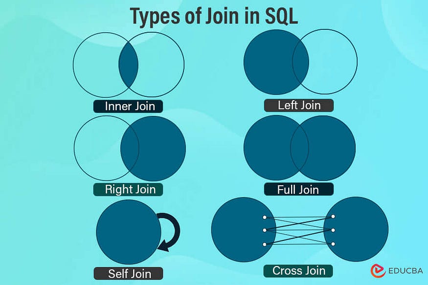
What is the difference between LEFT, RIGHT, FULL outer join and INNER join?

Joins

In order to understand this better, let’s consider two tables CONTINENTS and COUNTRIES as shown below. I shall show sample queries considering these two tables.

Table Name: CONTINENTS

Has data of 6 continents. Please note the continent “Antarctica” is intentionally missed from this table.

Table Name: COUNTRIES

Has data of one country from each continent. Please note that I have intentionally missed to add a country from Europe in this table.

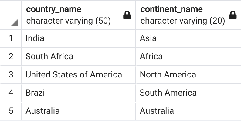
INNER JOIN will fetch only those records which are present in both the joined tables. The matching of the records is only based on the columns used for joining these two tables. INNER JOIN can also be represented as JOIN in your SELECT query.

INNER JOIN Query
SELECT cr.country_name, ct.continent_name
FROM continents ct
INNER JOIN countries cr
ON ct.continent_code = cr.continent_code;

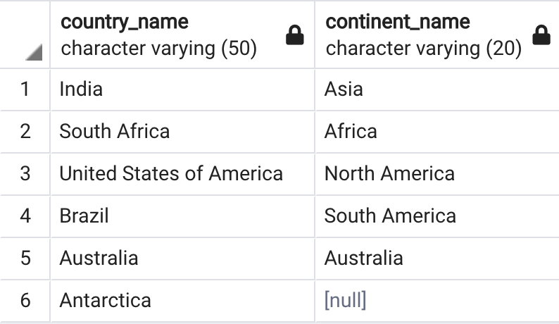
LEFT JOIN will fetch all records from the left table (table placed on the left side during the join) even if those records are not present in right table (table placed on the right side during the join). If your select clause has a column from the right table then for records which are not present in right table (but present in left table), SQL will return a NULL value. LEFT JOIN can also be represented as LEFT OUTER JOIN in your SELECT query.

LEFT JOIN Query
SELECT cr.country_name, ct.continent_name
FROM continents ct
LEFT JOIN countries cr
ON ct.continent_code = cr.continent_code;

RIGHT JOIN will fetch all records from the right table (table placed on the right side during the join) even if those records are not present in left table (table placed on the left side during the join). If your select clause has a column from the left table then for records which are not present in left table (but present in right table), SQL will return a NULL value. RIGHT JOIN can also be represented as RIGHT OUTER JOIN in your SELECT query.

*Note: LEFT and RIGHT join depends on whether the table is placed on the left side of the JOIN or on the right side of the JOIN.

RIGHT JOIN Query
SELECT cr.country_name, ct.continent_name
FROM continents ct
RIGHT JOIN countries cr
ON ct.continent_code = cr.continent_code;

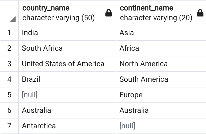
FULL JOIN will fetch all records from both left and right table. It’s kind of combination of INNER, LEFT and RIGHT join. Meaning FULL JOIN will fetch all the matching records in left and right table + all the records from left table (even if these records are not present in right table) + all the records from right table (even if these records are not present in left table). FULL JOIN can also be represented as FULL OUTER JOIN in your SELECT query.

FULL OUTER JOIN Query
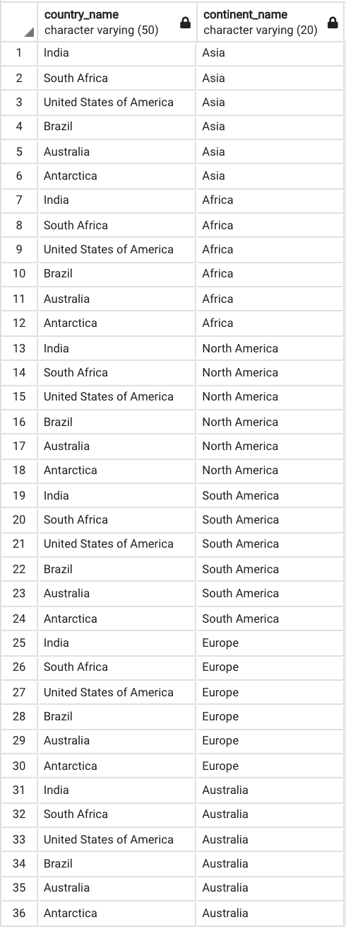
SELECT cr.country_name, ct.continent_name
FROM continents ct
FULL OUTER JOIN countries cr
on ct.continent_code = cr.continent_code;

Also check for what is SELF join, NATURAL join and CROSS join?

SELF JOIN is when you join a table to itself. There is no keyword like SELF when doing this join. We just use the normal INNER join to do a self join. Just that instead of doing an inner join with two different table, we inner join the same table to itself. Just that these tables should have different alias name. Other than this, SELF join performs similar to INNER join.

SELF JOIN Query
SELECT cr1.country_name
FROM countries cr1
JOIN countries cr2ON cr1.country_code = cr2.continent_code;

NATURAL JOIN is similar to INNER join but we do not need to use the ON clause during the join. Meaning in a natural join we just specify the tables. We do not specify the columns based on which this join should work. By default when we use NATURAL JOIN, SQL will join the two tables based on the common column name in these two tables. So when doing the natural join, both the tables need to have columns with same name and these columns should have same data type.

NATURAL JOIN Query
SELECT cr.country_name, ct.continent_name
FROM continents ct
NATURAL JOIN countries cr;

CROSS JOIN will join all the records from left table with all the records from right table. Meaning the cross join is not based on matching any column. Whether there is a match or not, cross join will return records which is basically number of records in left table multiplied by number of records in right table. In other words, cross join returns a Cartesian product.

CROSS JOIN Query
SELECT cr.country_name, ct.continent_name
FROM continents ct
CROSS JOIN countries cr;

## Question 10.

Can we use aggregate function as window function? If yes then how do we do it?

Yes, we can use aggregate function as a window function by using the OVER clause. Aggregate function will reduce the number of rows or records since they perform calculation of a set of row values to return a single value. Whereas window function does not reduce the number of records.

Now, let’s use the SUM function as a window function to calculate the running total salary within each department based on the order of salaries:

SELECT
employee_id,
employee_name,
department,
salary,
SUM(salary) OVER (PARTITION BY department ORDER BY salary) AS running_total_salary
FROM
employees;

Output:

| employee_id | employee_name | department | salary   | running_total_salary |
|-------------|---------------|------------|----------|-----------------------|
| 1 | John | HR | 50000.00 | 50000.00 |
| 3 | Bob | HR | 55000.00 | 105000.00 |
| 2 | Jane | IT | 60000.00 | 60000.00 |
| 4 | Alice | IT | 70000.00 | 130000.00 |

In this example, the running_total_salary column represents the running total salary within each department, calculated based on the ascending order of salaries. The PARTITION BY clause is used to partition the result set by the department column. The ORDER BY clause specifies the order of rows within each partition based on the salary column. The SUM function is applied as a window function, and it calculates the running total salary for each row within its department.

SQL is a powerful tool for managing and manipulating data in relational databases. While basic SQL queries are essential, mastering advanced SQL queries empowers data professionals to extract complex insights and perform sophisticated data transformations. In this article, we’ll explore 20 advanced SQL queries that cover a wide range of scenarios, from subqueries to window functions, with practical code examples.

Photo from Pexels

1. Subqueries

Subqueries allow us to nest one query inside another, enabling more complex data retrieval and filtering.

Example:

SELECT *
FROM employees
WHERE department_id IN (SELECT department_id FROM departments WHERE location_id = 1700);

2. Joins

SQL joins combine rows from two or more tables based on a related column between them.

Example:

SELECT e.employee_id, e.first_name, e.last_name, d.department_name
FROM employees e
JOIN departments d ON e.department_id = d.department_id;

3. Aggregate Functions

Aggregate functions perform calculations on a set of values and return a single value.

Example:

SELECT AVG(salary) AS avg_salary
FROM employees;

4. Window Functions

Window functions operate on a set of rows related to the current row within a query result.

Example:

SELECT employee_id, salary, 
AVG(salary) OVER (PARTITION BY department_id) AS avg_salary_by_dept
FROM employees;

5. Common Table Expressions (CTEs)

CTEs are temporary result sets that can be referenced within a SELECT, INSERT, UPDATE, or DELETE statement.

Example:

WITH high_salary_employees AS (
SELECT *
FROM employees
WHERE salary > 100000
)
SELECT * FROM high_salary_employees;

6. Pivot Tables

Pivot tables reorganize data from rows into columns, summarizing it in the

Must Watch YouTube Videos for Databricks Platform Administrators

  While written word is clearly the medium of choice for this platform, sometimes a picture or a video can be worth 1,000 words. Below are  ...