Optimising Output File Size in Apache Spark

 

A Comprehensive Guide on Managing Partitions, Repartition, and Coalesce Operations

Picture yourself at the helm of a large Spark data processing operation. One often-mentioned rule of thumb in Spark optimisation discourse is that for the best I/O performance and enhanced parallelism, each data file should hover around the size of 128Mb, which is the default partition size when reading a file [1].

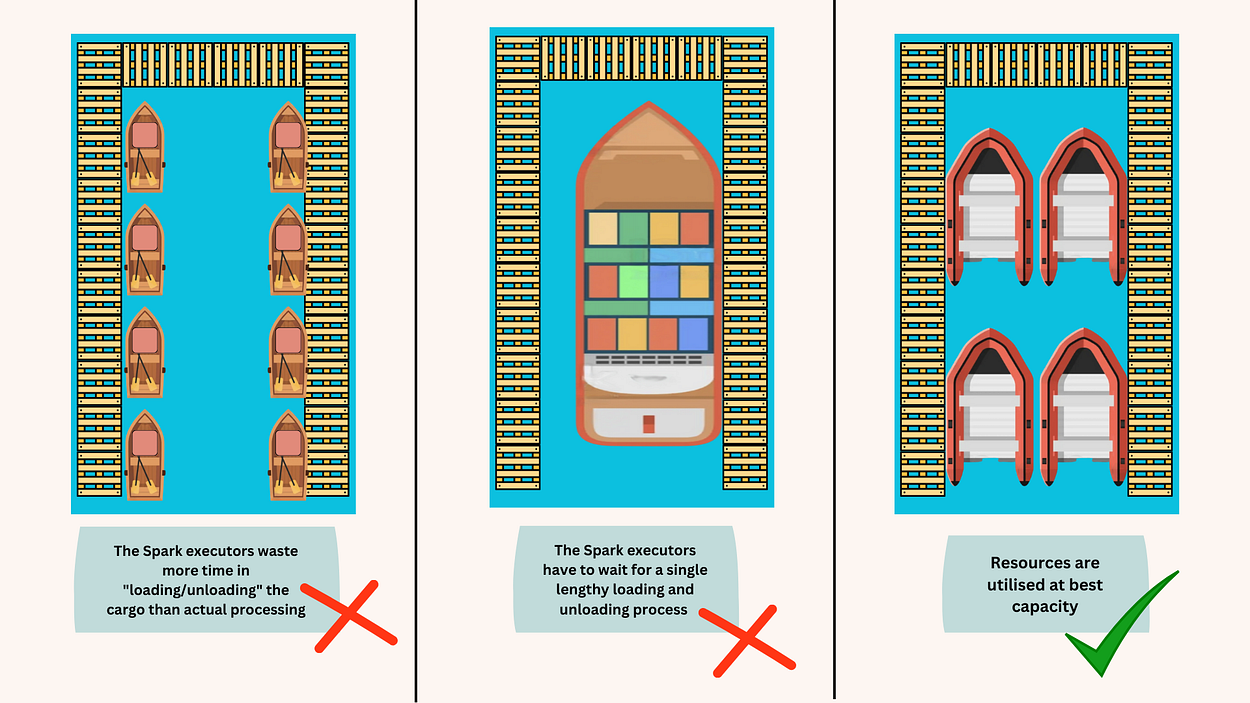
Imagine your files as vessels navigating the sea of data processing. If the vessels are too small, they waste a lot of time docking and setting sail again, a metaphor for the execution engine spending extra time opening files, listing directories, getting object metadata, setting up data transfer, and reading files. Conversely, if your vessels are too large and you don’t use the many docks of the port, they have to wait for a single lengthy loading and unloading process, a metaphor for the query processing waiting until a single reader has finished reading the entire file, which reduces parallelism [fig. 1].

Fig. 1 — Image by the author

To vividly illustrate the significance of file size optimisation, refer to the following figure. In this specific example, every table holds 8 GB of data.

However, navigating this delicate balance is no easy task, especially when dealing with large batch jobs. You may feel like you’ve lost control over the number of output files. This guide will help you regain it.

The Key to Understanding: Partitions

The number of output files saved to the disk is equal to the number of partitions in the Spark executors when the write operation is performed. However, gauging the number of partitions before performing the write operation can be tricky.

When reading a table, Spark defaults to read blocks with a maximum size of 128Mb (though you can change this with sql.files.maxPartitionBytes). Thus, the number of partitions relies on the size of the input. Yet in reality, the number of partitions will most likely equal the sql.shuffle.partitions parameter. This number defaults to 200, but for larger workloads, it rarely is enough. Check out this video to learn how to set the ideal number of shuffle partitions.

The number of partitions in Spark executors equals sql.shuffle.partitions if there is at least one wide transformation in the ETL. If only narrow transformations are applied, the number of partitions would match the number created when reading the file.

Setting the number of shuffle partitions gives us high-level control of the total partitions only when dealing with non-partitioned tables. Once we enter the territory of partitioned tables, changing the sql.shuffle.partitions parameter won’t easily steer the size of each data file.

The Steering Wheel: Repartition and Coalesce

We have two main ways to manage the number of partitions at runtime: repartition() and coalesce(). Here's a quick breakdown:

• Repartition: repartition(partitionCols, n_partitions) is a lazy transformation with two parameters - the number of partitions and the partitioning column(s). When performed, Spark shuffles the partitions across the cluster according to the partitioning column. However, once the table is saved, information about the repartitioning is lost. Therefore, this useful piece of information won’t be used when reading the file.

df = df.repartition("column_name", n_partitions)

• Coalesce: coalesce(num_partitions) is also a lazy transformation, but it only takes one argument - the number of partitions. Importantly, the coalesce operation doesn’t shuffle data across the cluster — therefore it’s faster than repartition. Also, coalesce can only reduce the number of partitions, it won’t work if trying to increase the number of partitions.

df = df.coalesce(num_partitions)

The primary insight to take away here is that using the coalesce method is generally more beneficial. That’s not to say that repartitioning isn’t useful; it certainly is, particularly when we need to adjust the number of partitions in a dataframe at runtime.

In my experience with ETL processes, where I deal with multiple tables of varying sizes and carry out complex transformations and joins, I’ve found that sql.shuffle.partitions doesn’t offer the precise control I need. For instance, using the same number of shuffle partitions for joining two small tables and two large tables in the same ETL would be inefficient — leading to an overabundance of small partitions for the small tables or insufficient partitions for the large tables. Repartitioning also has the added benefit of helping me sidestep issues with skewed joins and skewed data [2].

That being said, repartitioning is less suitable prior to writing the table to disk, and in most cases, it can be replaced with coalesce. Coalesce takes the upper hand over repartition before writing to disk for a couple of reasons:

1. It prevents an unnecessary reshuffling of data across the cluster.
2. It allows data ordering according to a logical heuristic. When using the repartition method before writing, data is reshuffled across the cluster, causing a loss in its order. On the other hand, using coalesce retains the order as data is gathered together rather than being redistributed.

Let’s see why ordering the data is crucial.

Order on the Horizon: Importance of Ordering Data

We mentioned above how when we apply the repartitionmethod, Spark won’t save the partitioning information in the metadata of the table. However, when dealing with big data, this is a crucial piece of information for two reasons:

1. It allows scanning through the table much more quickly at query time.
2. It allows better compression — if dealing with a compressible format (such as parquet, CSV, Json, etc). This is a great article to understand why.

The key takeaway is to order the data before saving. The information will be retained in the metadata, and it will be used at query time, making the query much faster.

Let’s now explore the differences between saving to a non-partitioned table and a partitioned table and why saving to a partitioned table requires some extra adjustments.

Managing File Size in Partitioned Tables

When it comes to non-partitioned tables, managing the number of files during the save operation is a direct process. Utilising the coalescemethod before saving will accomplish the task, regardless of whether the data is sorted or not.

# Example of using coalesce method before saving a non-partitioned table
df.coalesce(10).write.format("parquet").save("/path/to/output")

However, this method isn’t effective when handling partitioned tables, unless the data is arranged prior to coalescing. To grasp why this happens, we need to delve into the actions taking place within Spark executors when the data is ordered versus when it isn’t [fig.2].

Fig. 2 — Image by the author

Therefore, the standard process to save data to a partition table should be:

# Example of using coalesce method after ordering the data in a partitioned table
df.orderBy("columnName").coalesce(10).write.format("parquet").save("/path/to/output_partitioned")

Other Navigational Aids

Beyond repartition and coalesce, you might find maxnumberofrecords helpful. It's a handy method to prevent files from getting too large and can be used alongside the methods above.

df.write.option("maxRecordsPerFile", 50000).save("file_path")

Final Thoughts

Mastering file size in a Spark job often involves trial and error. It’s easy to overlook optimisation in an era where storage space is cheap and processing power is just a click away. But as tera and petabytes of data processing become the norm, forgetting these simple optimisation techniques can have significant costs in monetary, time, and environmental terms.

I hope this article empowers you to make efficient adjustments to your ETL processes. Like a seasoned sea captain, may you navigate the waters of Spark with confidence and clarity.