Spark Architecture was one of the toughest elements to grasp when initially learning about Spark. I think one of the main reasons is that there is a vast amount of information out there, but nothing which gives insight into all aspects of the Spark Ecosystem. This is most likely because, its complicated! There are so many fantastic resources out there, but not all are intuitive or easy to follow.
I am hoping this part of the series will help people who have very little knowledge of the topic understand how Spark Architecture is built, from the foundations up. We will also investigate how we can provide our Spark system with work and how that work is consumed and completed by the system in the most efficient way possible.
As promised, this section is going to be a little more heavy. So buckle yourself in, this is going to be fun!
Physical Spark Hierarchy:
To understand how Spark programs work, we need to understand how a Spark system is built, brick by brick (see what I did there). There are a number of different ways to set up a Spark system, but for this part in the series we will discuss one of the most popular ways to set it up.
Generally, a Spark system is built using a number of separate machines who all work together towards a common goal, this is referred to as a cluster or distributed system. For a system like this to work, we need to have a machine which manages the cluster as a whole. This machine is usually labelled as the driver node.
Driver Node
The Spark driver is used to orchestrate the whole Spark cluster, this means it will manage the work which is distributed across the cluster as well as what machines are available throughout the cluster lifetime.

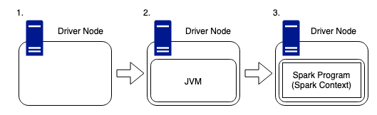
- The driver node is like any other machine, it has hardware such as a CPU, memory, DISKs and a cache, however, these hardware components are used to host the Spark Program and manage the wider cluster. The driver is the users link, between themselves, and the physical compute required to complete any work submitted to the cluster.
- As Spark is written in Scala, it is important to remember that any machine within the cluster needs to have a JVM (Java Virtual Machine) running, so that Spark can work with the hardware on the host.
- The Spark Program runs inside of this JVM and is used to create the SparkContext, which is the access point for the user to the Spark Cluster.
The driver contains the DAG (Directed Acyclic Graph) scheduler, task scheduler, backend scheduler and the block manager. These driver components are responsible for translating user code into Spark jobs executed on the cluster. Hidden away within the driver node is the cluster manager, which is responsible for acquiring resources on the Spark cluster and allocating them to a Spark job. These resources come in the form of worker nodes.
Worker Node(s)
Worker nodes form the “distributed” part of the cluster. These nodes come in all shapes and sizes and don’t always have to be the same to join a cluster, they can vary in size and performance. Although, having worker nodes which perform equally, can be a benefit when investigating performance bottlenecks further down the line. So, it’s something to bear in mind.

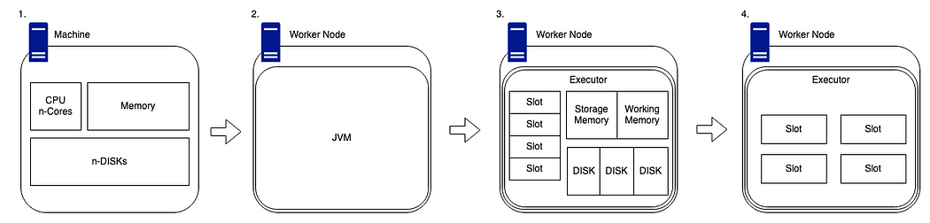
- Worker nodes are generally stand-alone machines which have hardware like any other. Such as a CPU, memory, disks and a cache.
- As with the driver, for Spark to run on a worker node, we need to ensure that the system has a compatible version of Java installed so that the code can be interpreted in the correct and meaningful way.
- When we have Spark installed on our worker node, our driver node will be able to utilise its cluster management capabilities to map what hardware is available on the worker.
The cluster manager will track the number of “slots”, which are essentially the number of cores available on the device. These slots are classified as available chucks of compute and they can be provided tasks to complete by the driver node.
There is an amount of available memory which is split into two sections, storage memory and working memory. The default ratio of this is 50:50, but this can be changed in the Spark config.
Each worker also has a number of disks attached. But I know what you are going to say, Spark works in memory, not disk! However, Spark still needs disks to allocate shuffle partitions (discussed further, later in this article), it also needs space for persistence to disk and also spill to disk. - Now we have the details of how Driver nodes and Worker nodes are structured, we need to know how that interact and deal with work.
For this we will create a minimalist version of the diagram to show a worker node and its available slots for work.
Minimised Physical Structure
Now that we know how the Driver and Workers are structured independently, we can look into how they are intrinsically linked within the context of a cluster. As stated above we will simplify the view of the worker node, such that it shows only the elements that are important for the next section. (They still have memory and disks!)
Looking at the Driver and Worker nodes we can see that the Driver node is the central hub for communication between nodes in the cluster.

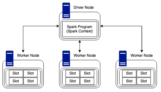
Worker nodes are able to communicate and pass data between each other but in regards to work and tasks, the Driver node is solely responsible for providing Workers with jobs to complete.
With the example above, we have a cluster containing a driver, and three worker nodes. Each node has four slots of compute available, so, this cluster would be able to complete twelve tasks in unison. It is worth mentioning that Sparks new photon engine is a Spark compatible vectorised query engine which has been developed to meet and take advantage of the latest CPU architecture. This enables faster parallel processing of data and even live performance improvements as data is read during task execution.
Spark Runtime Architecture
The Spark runtime architecture is exactly what it says on the tin, what happens to the cluster at the moment of code being run. Well, “code being run” might be the wrong phase. Spark has both eager and lazy evaluation. Spark actions are eager; however, transformations are lazy by nature.
As stated above, transformations are lazy, this essentially means when we call some operation on our data, it does not execute immediately. Spark maintains the record of which operation is being called. These operations can include joins and filters.
Actions are eager, which means that when an action is called, the cluster will start to compute the expected results as soon as the line of code is run. When Actions are run, they result in a non-RDD (resilient distributed dataset) component.
Types of Transformations:
There are two types of transformations which are key to understanding how Spark manages data and computes in a distributed manner, these are narrow and wide. Transformations create RDDs from each other.


- Narrow Transformations are defined by one input partition will result in one output partition. An example of this could be a filter: as we can have a data frame of data which we can filter down to a smaller dataset without the need to understand any data held on any other worker node.
- Wide transformations (shuffles) are defined by the fact the worker nodes will need to transfer (shuffle) data across the network to complete the required task. An example of this could be a join: as we may need to collect data from across the cluster to complete a join of two datasets fully and correctly.


Wide transformations can take many forms, and n input partitions may not always results in n output partitions. As stated above, joins are classed as wide transformations. So in the instance above, we have two RDD’s which have varying number of partitions being joined together to form a new RDD.
Runtime
When the user submits code to the driver via their preferred method, the driver implicitly converts the code containing transformations (filters, joins, groupby, unions, etc) and actions (counts, writes, etc) into an unresolved logical plan.
At the submission stage, the driver refers to the logical plan catalog to ensure all code conforms to the required parameters, after this is complete the unresolved logical plan is tranformed into a logical plan. The process now performs optimisations, like planning transformations and actions, this optimiser is better know as the catalyst optimiser.
At the core of Spark SQL is the Catalyst optimizer, which leverages advanced programming language features (e.g. Scala’s pattern matching and quasi quotes) in a novel way to build an extensible query optimizer. Catalyst is based on functional programming constructs in Scala and designed with these key two purposes:
- Easily add new optimization techniques and features to Spark SQL
- Enable external developers to extend the optimizer (e.g. adding data source specific rules, support for new data types, etc.)


I will be doing a deep dive into the catalyst optimiser in the next part of the series, so don’t worry about that part too much.
Once the optimisations are complete, the logical plan is converted into multiple physical execution plans, these plans are funnelled into a cost model with analyses each plan and applies a cost value to run each execution plan. The plan with the lowest cost to complete will be selected as the final output. This selected execution plan will contain job(s) with multiple stages.

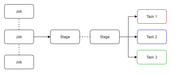
Stages have small physical called tasks which are bundled to be sent to the Spark cluster. Before these tasks are distributed, the driver program talks to the cluster manager to negotiate for resources.

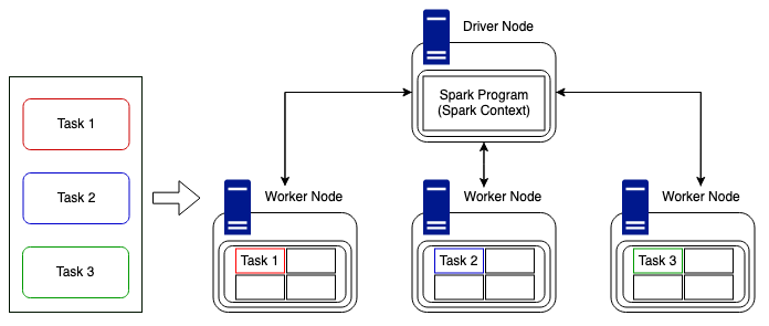
Once this is done and resources have been allocated, tasks are distributed to the worker nodes (executors) who have free time, and the driver program monitors the progress. This is done in the most efficient way possible keeping in mind the current available resources and the cluster structure. In the above example it is simple, we have three tasks to distribute to three worker nodes. Tasks could be distributed in the way above, i.e. one task to each worker node, or they could be sent to one node and still run asynchronously due to the parallel nature of Spark. But complexity arises when we have more tasks than available slots of compute, or when we have a non uniformly divisible number of tasks compared to that of the nodes in the cluster. Luckily for us, Spark deals with this itself and manages the task distribution.
It is worth mentioning, although Spark can distribute tasks in and efficient way, it cannot always interpret the data, meaning, we could encounter data skew which can cause vast time differences in task duration. However, this all depends on how the underlying data lake is structured. If it is built using Delta Engine (Photon) we can take advantage of the live improvement to query execution as well as improvements which encourage better shuffle sizes and optimal join types.
The Spark UI (user interface) allows the user to interogate the entire workload process, meaning the user can dive into each part. For example, there are tabs for Jobs and Stages. By moving into a stage the user can look at metrics related to specific tasks, this method can be used to understand why specific jobs may be taking longer than expected to complete.
Cloud vs Local
As I am sure you have guessed, Spark clusters are generally built within a cloud environment using popular services from cloud service providers. This is done due to the scalability, reliability and cost effectiveness of these services. However, you may not be aware that you can run Spark on your local machine if you want to play around with the Spark config.
By far the easiest option for tinkering, is to sign up to the community edition of Databricks. This allows you to create a small but reasonably powerful single worker node cluster with the capability to run all of the Databricks code examples and notebooks. If you haven’t done it already… do it! There are limitations and the clusters do timeout after two hours of idle time, but free compute is free compute!
Finally
Spark Architecture is hard. It takes time to understand the physical elements, and how the core runtime code translates into data being transformed and moving around a cluster. As we work through the series, we will continue to refer back to this section to ensure we all have the fundamentals locked into our grey matter.
For this series, I will be looking into ways that we will be able to dive even deeper into the depths of Spark such that we can understand the bare bones of the JVM structurre and how the optimisers function on our unresolved logical plans.
It is worth noting that there will be an upcoming section, where we will be building a Spark cluster using a Raspberry Pi as the Driver node, and a number of Raspberry Pi Zero’s as the Worker Nodes. I just need to wait for the items to be delivered… Covid delivery times are slow!
If I have missed anything from this section, or if something still isn’t clear, please let me know so that I can improve this series and not to mention my Spark knowledge! You can find me on LinkedIn:


No comments:
Post a Comment