PyTorch : A Deep Learning Framework

Part 1 — What are Tensors and Gradients?

---

PyTorch is a open source, deep learning framework developed by Facebook.

INSTALLATION OF PYTORCH

The installation of PyTorch Package is done either through pip manager or conda command.

I would recommend using Google Colab as our IDE . PyTorch can be used by directly importing torch package

import torch# importing pytorch library in Google Colab# pip install torch===1.5.0 torchvision===0.6.0 -f https://download.pytorch.org/whl/torch_stable.html# Through pip installation# !conda install pytorch cpuonly -c pytorch -y# Through Conda Installation

WHAT IS A TENSOR?

The main element of PyTorch is PyTorch Tensor.

Tensor is a type of data structure in Linear Algebra represented in the form of multi-dimensional array. It can be a scalar, vector , matrix or any n dimension array.

Whenever a library is imported in Python it is treated as an object. Object has 2 important features.

1. Methods
2. Attributes

NOTE: To define a PyTorch tensor, torch.tensor() method is used and .ndim, .dtype are some of its attributes.

DEFINING A 0D TENSOR — ONLY A NUMBER

Fig 2 : Zero Dimension Tensor(Only a Single Number)

Scalar consists of a single value. It is then printed to view the tensor. Also, ndim and dtype attributes are used to check the dimension of the tensor and the datatype of that respective tensor

Fig 3: One Dimension Tensor(Vector)

One Dimension Tensor can also be called as a Vector. It has got one dimension.

Fig 4: Accessing the values of Tensor

The contents of the Tensor can be accessed just like how we access the values of a list.

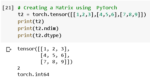
Fig 5: 2 Dimension Tensor(Matrix)

Fig 6 : Comparison of shape attribute between 0D, 1 D and 2 D Tensor

Shape of N — Dimension Array

Here the shape of the Tensor is (4,2,3). Lets break this torch.size value.

4 indicates the total number of values in the outer dimension.

2 indicates the total number of values in 2nd Dimension. In this case it mentions the number of rows in the inner matrix.

3 indicates the number of values in the inner dimesion. In this case it is the number of columns in the inner matrix.

So to conclude, the tensor consists of totally 4 matrices with 2 rows and 3 columns.

.requires_grad = True

We need to calculate the partial derivative on a respective tensor to change the values of weights and bias in Backpropogation method. Now, to calculate the derivative of tensors with large number of dimension is impractical to calculate. Hence, we use the parameter .requires_grad to find the gradient.

Fig : Parameter for calculating Gradient of a Tensor

NOTE: Please make sure that the dtype of Tensor is floating point for calculating Gradients.

HOW TO PRINT THE VALUES OF GRADIENTS?

In Neural Network, we often come across the terms weights and bias. They can be compared to slope and co-efficient value in an equation of a straight line. We basically multiply weight with the independent value or input and and the combined value with the bias.

Let us take 3 sensors names input_value, weight_value and bias_value with scalar value

input_value = torch.tensor(2.3,requires_grad=True)weight_value = torch.tensor(2.0,requires_grad=True)bias_value = torch.tensor(0.45,requires_grad=True)

Lets calculate the output by taking product of weight with input and adding the combined value with bias as in the case of equation of straight line.

output_value = weight_value*input_value+bias_valueprint(output_value)

Fig : Use Backward method to display gradients

The output_value is as shown, but to print the gradients of each value we have call for backward method. This can be written as

output_value.backward()

Now, time to print the output of gradients.

# Display gradientsprint('dy/dx:', input_value.grad)print('dy/dw:', weight_value.grad)print('dy/db:', bias.grad)

In the next part, we will discuss few interesting methods of PyTorch library.

I had mentioned in my previous blog regarding the operations of Tensors. We will be covering few of the interesting operations of Tensors.

1. Stride Operation on Tensors

Strides are the number of steps needed to go from one location to another in a given dimension of a Matrix.

First let me import the torch library and create a tensor using randn method having dimension of 3 rows and 2 columns

import torcht0 = torch.randn(3,2)t0

Output of t1 tensor

Now taking stride operator we get the output in the form of tuple

t0.stride()>>> (2,1)

This resultant tuple tells us the following:

1. If you want to move along with axis = 0 (or vertically), lets say we want to jump from -0.1868 to -0.0640 , you need to move 2 steps
2. If you want to move along with axis =1( or horizontally),lets say we want to jump from -0.1868 to -0.8337, you need to move only 1 step

Lets consider using as_strided() now,

Syntax : torch.as_strided(input, size, stride, storage_offset=0) → Tensor

t1 = torch.as_strided(t0,(2,1),(4,2),1)t1>>> tensor([[-0.8337],
            [ 0.9209]])

Here input is t0 which we had defined earlier.

Next output Tensor size is (2,1).

Stride is (4,2). Since we have only 1 output column, we will consider only the stride value for axis = 1(to move along the rows) which is 4

Offset value is given as 1 which means the starting value will be at index 0 i.e., -0.8337

Then take 4 steps as mentioned in the stride. The next value will be at index 5 which is 0.9209

Another example,

t2 = torch.as_strided(t0,(2,2),(3,2),0)t2>>> tensor([[-0.1868, -0.0640],     
            [ 0.1071,  0.9209]])

In this example, input source is again t0,

Output Tensor shape: (2,2)

Stride Value(3,2)

Offset Value : 0 [ That’s why starting value will be -0.1868]

Since the Shape of Output Tensor contains 2 rows and 2 columns, we will have to traverse along the axis = 0 as well as axis =1.

For mentioning the value with index 1 of output tensor, we need to consider the stride value of 2, which will be index 3 of t0 .i.e,-0.0640

Taking next the stride value of 3 from -0.1868 , we get 0.1071

Finally taking again stride value of 2 from 0.1071, we get 0.9209 as final value.

Considering a different example now,

t3 = torch.as_strided(t0,(3,3),(1,2))t3

We get the above RuntimeError mentioning the wrong dimension of output tensor.

2. Quantized Tensor

Quantization of Tensor is a process of scaling the values of tensors in one particular range

Syntax: torch.quantize_per_tensor(input, scale, zero_point, dtype) → Tensor

Example 1:

torch.quantize_per_tensor(torch.tensor([-0.5, 0.5, 1.0, 2.0]), 0.2, 5, torch.quint8).int_repr()>>> tensor([ 2,  8, 10, 15], dtype=torch.uint8)

The values -0.5, 0.5, 1.0, 2.0 are scaled to integer values for scaling value of 0.2

Example 2:

torch.quantize_per_tensor(torch.tensor([-15, 5, -10, 20]), 0.2, 100, torch.quint8).int_repr()

3. Non Zero Index Tensor

This method returns an index value in the form of tensor of non zero elements. The input source will be again considered as a tensor.

Example -1

torch.nonzero(torch.tensor([1,2,3,0,6,0,9.8]))>>> tensor([[0],         
            [1],         
            [2],         
            [4],         
            [6]])

Clearly from the above example, we can demonstrate that non-zero elements are found in index 0,1,2,4 and 6

Example — 2

torch.nonzero(torch.tensor([[1,0,0,0],[1,0,0,1]]))>>> tensor([[0, 0],         
            [1, 0], 
            [1, 3]])

There are non- zero elements in the above tensor and the respective indices are formed as the values of the output tensor

Example — 3

torch.nonzero(torch.tensor(['A',0,1]))

The nonzero method wont support String values. Using ord function to get ASCII number of A would a great option.

4. Condition on Tensor using where

The operation is defined as:

Return a tensor of elements selected from either x or y, depending on condition.

x = 12.5*torch.randn(4,5)y = torch.zeros(1)x>>>tensor([[ -3.9482,  -9.9197,   1.3945,  13.3218, -15.9004],                     [ -9.2214,  21.2780,  -0.4671,  -2.4064,   5.6129],           [-14.5062,  26.1567,   4.9364,   5.1095,  10.4315],         
[ -3.5484,  22.1428,   0.9145,  -1.0481, -14.0949]])

I am taking 12.5 constant to multiply with all the values of tensors using broadcasting. This is done to get a higher range random value.

Example — 1

torch.where(x>0,x,y)>>>tensor([[ 0.0000,  0.0000,  1.3945, 13.3218,  0.0000],         [ 0.0000, 21.2780,  0.0000,  0.0000,  5.6129],        
[ 0.0000, 26.1567,  4.9364,  5.1095, 10.4315],         
[ 0.0000, 22.1428,  0.9145,  0.0000,  0.0000]]

Accepting only positive value, negative values are replaced with zeros

Example — 2

torch.where(x>0,x,torch.round(x))>>>tensor([[ -4.0000, -10.0000,   1.3945,  13.3218, -16.0000],         [ -9.0000,  21.2780,  -0.0000,  -2.0000,   5.6129],         [-15.0000,  26.1567,   4.9364,   5.1095,  10.4315],         
[ -4.0000,  22.1428,   0.9145,  -1.0000, -14.0000]])

All negative values to be rounded to nearest Integer and positive values printed as it is.

Example — 3

torch.where((x>0.5) and (x <1.0),x,y)

5. Scatter method on Tensor

Writes all the values from source to the output tensor based on indexing.

Syntax: scatter_(dim, index, src) → Tensor

Example — 1

torch.zeros(3, 5).scatter_(0, torch.tensor([[0,1,1,1,1],[1,0,1,0,0]]), 14)>>>tensor([[14., 14.,  0., 14., 14.],         
          [14., 14., 14., 14., 14.],         
          [ 0.,  0.,  0.,  0.,  0.]])

The parameter dim which is 0 in our case tells the axis along which we have to index

Here the source value is given as 14

Consider replacing value 14 with the index values[0,1,1,1,1] and [1,0,1,0,0].

If you observe all the elements are replaced with 14 except one because, there is no mention of index 0 in the 3rd term of both the indices

Example — 2

torch.zeros(2,2).scatter(1,torch.tensor([[1,0],[0,1]]),12)>>> tensor([[12., 12.],
           [12., 12.]])

Replacing 12 with all index values.

Above were few of the interesting Tensor operations in PyTorch.

The link for Google Colab Notebook is as follows:

https://github.com/diazonic/pytorch/blob/master/PyTorch_Part_2_Tensors_Operations.ipynb

In the upcoming blog, I will be covering Linear Regression and the concept of Gradient Descent in Deep Learning using PyTorch