Saturday, May 30, 2020

NumPy Crash Course: Array Basics

Lists vs. Arrays

We’re all familiar with the standard Python list — a mutable object that has great flexibility in that not all elements of the list need to be of a homogeneous data type. That is, you can have a list containing integers, strings, floats, and even other objects.
my_list = [2, {'dog': ['Rex', 3]}, 'John', 3.14]
The above is a perfectly valid list containing multiple data types as elements — even a dictionary which contains another list!
However, to support all these simultaneous data types, each Python list element must contain its own unique information. Each element acts as a pointer to a unique Python Object. Because of this inefficiency, it becomes much more taxing to use lists as they grow larger and larger.
>>>for element in my_list:
    print(type(element))<class 'int'>
<class 'dict'>
<class 'str'>
<class 'float'>
With an array, we do away with the flexibility of lists and instead, we have a multidimensional table of elements of the same data type (generally integers).
This allows for much more efficient storage and manipulation of large data sets.

Properties of Arrays

Each dimension of the NumPy array is known as an axis. For example, if we declared an array as follows we have an array on 2 axes:
>>> import numpy as np
>>> a = np.arange(10).reshape(2,5)
>>> a
array([[0, 1, 2, 3, 4],
       [5, 6, 7, 8, 9]])
The above code uses the arrange() function to create an array of range 10 and reshapes it to be a 2 x 5 array. This method is just the array version of the standard range() function.
You can see properties of your array uses the built-in array attributes shape, ndim, dtype, itemsize, and size.
>>> # Returns a tuple of the size of each dimension
>>> a.shape
(2, 5)>>> # Returns the number of axes of the array
>>> a.ndim
2>>> # Returns the description of the data type of the array
>>> a.dtype
dtype('int32')>>> # Returns the byte size of each element in the array
>>> a.itemsize
4>>> # Returns the total number of elements in the array
>>> a.size
10

Creating Arrays

There is a whole host of ways you can create NumPy arrays from scratch — it will generally depend on your application as to which method to use, but some of the more common techniques are outlined below.
Note: the dtype parameter is optional if you want to specify the type explicitly, otherwise it will default to a type most appropriate to the data you pass at the time of creation.
>>> # Create an array of specified size filled with 0's
>>> np.zeros((3,3), dtype=int)
array([[0, 0, 0],
       [0, 0, 0],
       [0, 0, 0]])>>> # Create an array of specified size filled with the given value
>>> np.full((4,2), 1.23)
array([[1.23, 1.23],
       [1.23, 1.23],
       [1.23, 1.23],
       [1.23, 1.23]])>>> # Create a linear array with values from the arange() function
>>> np.arange(10)
array([0, 1, 2, 3, 4, 5, 6, 7, 8, 9])>>> # Create an array of N evenly spaced values between x and y
>>> # np.linspace(x, y, N)
array([0.        , 0.11111111, 0.22222222, 0.33333333, 0.44444444,
       0.55555556, 0.66666667, 0.77777778, 0.88888889, 1.        ])>>> # Create an array of random values between 0 and 1
>>> np.random.random((2,2))
array([[0.90416154, 0.56633881],
       [0.09384551, 0.23539769]])>>> # Create an array of random integers between a given range
>>> np.random.randint(0, 5, (2,2))
array([[4, 3],
       [3, 3]])

Reshaping Arrays

You have already seen us make use of reshape() method and it can be extremely useful for manipulating your arrays. For some functions such as arange() and linspace(), you can use reshape() to create an array in whatever size desired.
However, it is very important to note that to be able to reshape an array, the size of the new array must match that of the original array. For example, the following is not a valid reshape:
>>> b = np.arange(0, 6)
>>> b
array([0, 1, 2, 3, 4, 5])
>>> b.reshape((3,3))Traceback (most recent call last):
  File "<pyshell#40>", line 1, in <module>
    b.reshape((3,3))
ValueError: cannot reshape array of size 6 into shape (3,3)
We have 6 elements, but are trying to reshape into a 3 x 3, which would require 9 elements. We could, however, reshape into a 3 x 2:
>>> b.reshape((3,2))
array([[0, 1],
       [2, 3],
       [4, 5]])
We can also ‘flatten’ the multidimensional array into a single dimension through using the ravel() method:
>>> b.ravel()
array([0, 1, 2, 3, 4, 5])

Indexing/Slicing Arrays

Array indexing works very similarly to list indexing and slicing, we just need to be mindful of the dimensionality of our data.
For example, suppose we were working with the array as shown below:
>>> x = np.arange(12).reshape((4,3))
>>> x
array([[ 0, 1, 2],
       [ 3, 4, 5],
       [ 6, 7, 8],
       [ 9, 10, 11]])
We have a 4 x 3 containing 12 elements in total. To access an element, we need to do so using a tuple. So, if we wanted to return a value in our multidimensional array, we would do it as such:
>>> # Return an entire axis
>>> x[0]
array([0, 1, 2])>>> # Return a specific element
>>> x[3][1]
10
We can use this to modify values in our array as well.
Note that if you try modifying the value to a data type different from your array, you can run into issues! Our float gets converted to an int when we try to modify an array of type int.
>>> # Modify a value using a correct data type
>>> x[1][1] = 30
>>> x
array([[ 0,  1,  2],
       [ 3, 30,  5],
       [ 6,  7,  8],
       [ 9, 10, 11]])>>> # Modify a value using an incorrect data type
>>> x[0][1] = 3.14
>>> x
array([[ 0,  3,  2],
       [ 3, 30,  5],
       [ 6,  7,  8],
       [ 9, 10, 11]])
For slicing, we again make use of the familiar list slicing notation, but when we deal with arrays of more than one dimension you separate each dimension with a comma.
We access the rows, and columns using the usual x[start:stop:step] format.
>>> x
array([[ 0,  3,  2],
       [ 3, 30,  5],
       [ 6,  7,  8],
       [ 9, 10, 11]])>>> # Return a slice of the first 2 rows and all columns
>>> x[:2, :]
array([[ 0,  3,  2],
       [ 3, 30,  5]])>>> # Return a slice of all rows up to the first column
>>> x[:, :1]
array([[0],
       [3],
       [6],
       [9]])>>> # Return every other row, every column
>>> x[::2, :]
array([[0, 3, 2],
       [6, 7, 8]])
Now that you have the basics of arrays under your belt, you’re well on your way to understanding one of the most powerful data structure in Python!
Next up, we’ll look at basic operations on arrays, so be sure to follow along with this series as it progresses.
Links to future stories will be added — along with an index page — as they are released.

Friday, May 29, 2020

PyTorch : A Deep Learning Framework

Part 1 — What are Tensors and Gradients?


PyTorch is a open source, deep learning framework developed by Facebook.

INSTALLATION OF PYTORCH

The installation of PyTorch Package is done either through pip manager or conda command.
I would recommend using Google Colab as our IDE . PyTorch can be used by directly importing torch package
import torch# importing pytorch library in Google Colab# pip install torch===1.5.0 torchvision===0.6.0 -f https://download.pytorch.org/whl/torch_stable.html# Through pip installation# !conda install pytorch cpuonly -c pytorch -y# Through Conda Installation

WHAT IS A TENSOR?

The main element of PyTorch is PyTorch Tensor.
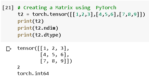
Tensor is a type of data structure in Linear Algebra represented in the form of multi-dimensional array. It can be a scalar, vector , matrix or any n dimension array.
Whenever a library is imported in Python it is treated as an object. Object has 2 important features.
  1. Methods
  2. Attributes
NOTE: To define a PyTorch tensor, torch.tensor() method is used and .ndim, .dtype are some of its attributes.

DEFINING A 0D TENSOR — ONLY A NUMBER

Scalar consists of a single value. It is then printed to view the tensor. Also, ndim and dtype attributes are used to check the dimension of the tensor and the datatype of that respective tensor
One Dimension Tensor can also be called as a Vector. It has got one dimension.
The contents of the Tensor can be accessed just like how we access the values of a list.
Here the shape of the Tensor is (4,2,3). Lets break this torch.size value.
4 indicates the total number of values in the outer dimension.
2 indicates the total number of values in 2nd Dimension. In this case it mentions the number of rows in the inner matrix.
3 indicates the number of values in the inner dimesion. In this case it is the number of columns in the inner matrix.
So to conclude, the tensor consists of totally 4 matrices with 2 rows and 3 columns.

.requires_grad = True

We need to calculate the partial derivative on a respective tensor to change the values of weights and bias in Backpropogation method. Now, to calculate the derivative of tensors with large number of dimension is impractical to calculate. Hence, we use the parameter .requires_grad to find the gradient.
Error
NOTE: Please make sure that the dtype of Tensor is floating point for calculating Gradients.

HOW TO PRINT THE VALUES OF GRADIENTS?

In Neural Network, we often come across the terms weights and bias. They can be compared to slope and co-efficient value in an equation of a straight line. We basically multiply weight with the independent value or input and and the combined value with the bias.
Let us take 3 sensors names input_value, weight_value and bias_value with scalar value
input_value = torch.tensor(2.3,requires_grad=True)weight_value = torch.tensor(2.0,requires_grad=True)bias_value = torch.tensor(0.45,requires_grad=True)
Lets calculate the output by taking product of weight with input and adding the combined value with bias as in the case of equation of straight line.
output_value = weight_value*input_value+bias_valueprint(output_value)
The output_value is as shown, but to print the gradients of each value we have call for backward method. This can be written as
output_value.backward()
Now, time to print the output of gradients.
# Display gradientsprint('dy/dx:', input_value.grad)print('dy/dw:', weight_value.grad)print('dy/db:', bias.grad)
In the next part, we will discuss few interesting methods of PyTorch library.

I had mentioned in my previous blog regarding the operations of Tensors. We will be covering few of the interesting operations of Tensors.

1. Stride Operation on Tensors

Strides are the number of steps needed to go from one location to another in a given dimension of a Matrix.
First let me import the torch library and create a tensor using randn method having dimension of 3 rows and 2 columns
import torcht0 = torch.randn(3,2)t0
Now taking stride operator we get the output in the form of tuple
t0.stride()>>> (2,1)
This resultant tuple tells us the following:
  1. If you want to move along with axis = 0 (or vertically), lets say we want to jump from -0.1868 to -0.0640 , you need to move 2 steps
  2. If you want to move along with axis =1( or horizontally),lets say we want to jump from -0.1868 to -0.8337, you need to move only 1 step
Lets consider using as_strided() now,
Syntax : torch.as_strided(inputsizestridestorage_offset=0) → Tensor
t1 = torch.as_strided(t0,(2,1),(4,2),1)t1>>> tensor([[-0.8337],
            [ 0.9209]])
Here input is t0 which we had defined earlier.
Next output Tensor size is (2,1).
Stride is (4,2). Since we have only 1 output column, we will consider only the stride value for axis = 1(to move along the rows) which is 4
Offset value is given as 1 which means the starting value will be at index 0 i.e., -0.8337
Then take 4 steps as mentioned in the stride. The next value will be at index 5 which is 0.9209
Another example,
t2 = torch.as_strided(t0,(2,2),(3,2),0)t2>>> tensor([[-0.1868, -0.0640],     
            [ 0.1071,  0.9209]])
In this example, input source is again t0,
Output Tensor shape: (2,2)
Stride Value(3,2)
Offset Value : 0 [ That’s why starting value will be -0.1868]
Since the Shape of Output Tensor contains 2 rows and 2 columns, we will have to traverse along the axis = 0 as well as axis =1.
For mentioning the value with index 1 of output tensor, we need to consider the stride value of 2, which will be index 3 of t0 .i.e,-0.0640
Taking next the stride value of 3 from -0.1868 , we get 0.1071
Finally taking again stride value of 2 from 0.1071, we get 0.9209 as final value.
Considering a different example now,
t3 = torch.as_strided(t0,(3,3),(1,2))t3
We get the above RuntimeError mentioning the wrong dimension of output tensor.

2. Quantized Tensor

Quantization of Tensor is a process of scaling the values of tensors in one particular range
Syntax: torch.quantize_per_tensor(inputscalezero_pointdtype) → Tensor
Example 1:
torch.quantize_per_tensor(torch.tensor([-0.5, 0.5, 1.0, 2.0]), 0.2, 5, torch.quint8).int_repr()>>> tensor([ 2,  8, 10, 15], dtype=torch.uint8)
The values -0.5, 0.5, 1.0, 2.0 are scaled to integer values for scaling value of 0.2
Example 2:
torch.quantize_per_tensor(torch.tensor([-15, 5, -10, 20]), 0.2, 100, torch.quint8).int_repr()

3. Non Zero Index Tensor

This method returns an index value in the form of tensor of non zero elements. The input source will be again considered as a tensor.
Example -1
torch.nonzero(torch.tensor([1,2,3,0,6,0,9.8]))>>> tensor([[0],         
            [1],         
            [2],         
            [4],         
            [6]])
Clearly from the above example, we can demonstrate that non-zero elements are found in index 0,1,2,4 and 6
Example — 2
torch.nonzero(torch.tensor([[1,0,0,0],[1,0,0,1]]))>>> tensor([[0, 0],         
            [1, 0], 
            [1, 3]])
There are non- zero elements in the above tensor and the respective indices are formed as the values of the output tensor
Example — 3
torch.nonzero(torch.tensor(['A',0,1]))
The nonzero method wont support String values. Using ord function to get ASCII number of A would a great option.

4. Condition on Tensor using where

The operation is defined as:
Return a tensor of elements selected from either x or y, depending on condition.
x = 12.5*torch.randn(4,5)y = torch.zeros(1)x>>>tensor([[ -3.9482,  -9.9197,   1.3945,  13.3218, -15.9004],                     [ -9.2214,  21.2780,  -0.4671,  -2.4064,   5.6129],           [-14.5062,  26.1567,   4.9364,   5.1095,  10.4315],         
[ -3.5484,  22.1428,   0.9145,  -1.0481, -14.0949]])
I am taking 12.5 constant to multiply with all the values of tensors using broadcasting. This is done to get a higher range random value.
Example — 1
torch.where(x>0,x,y)>>>tensor([[ 0.0000,  0.0000,  1.3945, 13.3218,  0.0000],         [ 0.0000, 21.2780,  0.0000,  0.0000,  5.6129],        
[ 0.0000, 26.1567,  4.9364,  5.1095, 10.4315],         
[ 0.0000, 22.1428,  0.9145,  0.0000,  0.0000]]
Accepting only positive value, negative values are replaced with zeros
Example — 2
torch.where(x>0,x,torch.round(x))>>>tensor([[ -4.0000, -10.0000,   1.3945,  13.3218, -16.0000],         [ -9.0000,  21.2780,  -0.0000,  -2.0000,   5.6129],         [-15.0000,  26.1567,   4.9364,   5.1095,  10.4315],         
[ -4.0000,  22.1428,   0.9145,  -1.0000, -14.0000]])
All negative values to be rounded to nearest Integer and positive values printed as it is.
Example — 3
torch.where((x>0.5) and (x <1.0),x,y)

5. Scatter method on Tensor

Writes all the values from source to the output tensor based on indexing.
Syntax: scatter_(dimindexsrc) → Tensor
Example — 1
torch.zeros(3, 5).scatter_(0, torch.tensor([[0,1,1,1,1],[1,0,1,0,0]]), 14)>>>tensor([[14., 14.,  0., 14., 14.],         
          [14., 14., 14., 14., 14.],         
          [ 0.,  0.,  0.,  0.,  0.]])
The parameter dim which is 0 in our case tells the axis along which we have to index
Here the source value is given as 14
Consider replacing value 14 with the index values[0,1,1,1,1] and [1,0,1,0,0].
If you observe all the elements are replaced with 14 except one because, there is no mention of index 0 in the 3rd term of both the indices
Example — 2
torch.zeros(2,2).scatter(1,torch.tensor([[1,0],[0,1]]),12)>>> tensor([[12., 12.],
           [12., 12.]])
Replacing 12 with all index values.
Above were few of the interesting Tensor operations in PyTorch.
The link for Google Colab Notebook is as follows:
In the upcoming blog, I will be covering Linear Regression and the concept of Gradient Descent in Deep Learning using PyTorch

Must Watch YouTube Videos for Databricks Platform Administrators

  While written word is clearly the medium of choice for this platform, sometimes a picture or a video can be worth 1,000 words. Below are  ...