Social networks are among the biggest sources of data today, and this means they are an extremely valuable asset for marketers, big data specialists, and even individual users like journalists and other professionals. Harnessing the potential of real-time Twitter data is also useful in many time-sensitive business processes. In this article, Toptal Freelance Software Engineer Hanee' Medhat explains how you can build a simple Python application to leverage the power of Apache Spark, and then use it to read and process tweets to identify trending hashtags.

 version of this article translated by Marisela Ordaz
Nowadays, data is growing and accumulating faster than ever before. Currently, around 90% of all data generated in our world was generated only in the last two years. Due to this staggering growth rate, big data platforms had to adopt radical solutions in order to maintain such huge volumes of data.
One of the main sources of data today are social networks. Allow me to demonstrate a real-life example: dealing, analyzing, and extracting insights from social network data in real time using one of the most important big data echo solutions out there—Apache Spark, and Python.

In this article, I’ll teach you how to build a simple application that reads online streams from Twitter using Python, then processes the tweets using Apache Spark Streaming to identify hashtags and, finally, returns top trending hashtags and represents this data on a real-time dashboard.
Creating Your Own Credentials for Twitter APIs
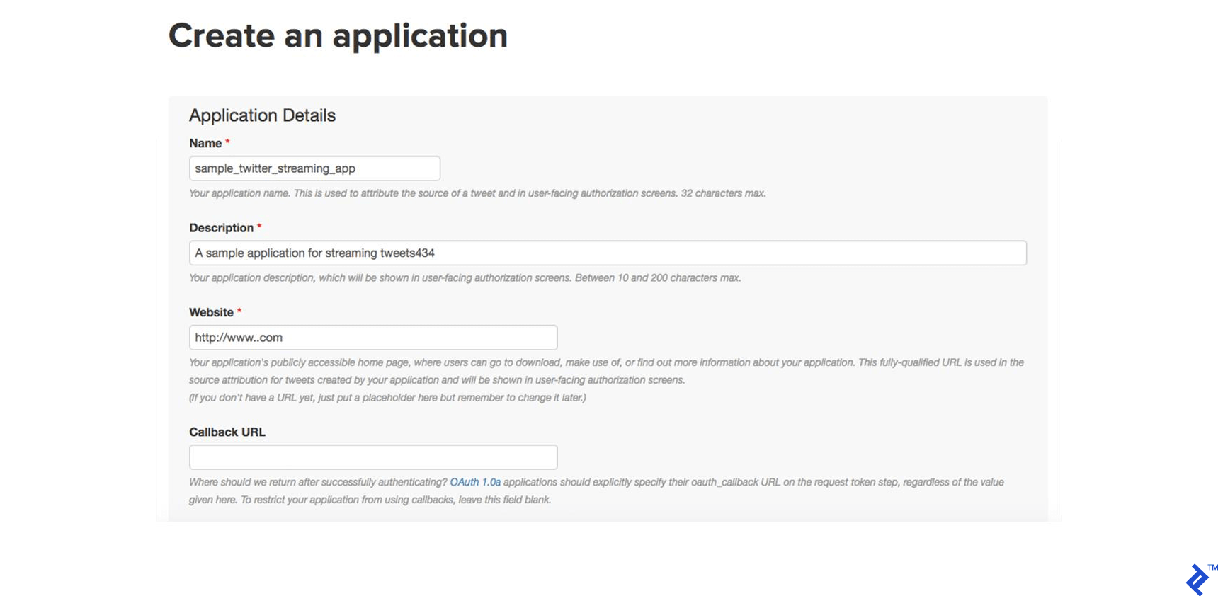
In order to get tweets from Twitter, you need to register on TwitterApps by clicking on “Create new app” and then fill the below form click on “Create your Twitter app.”
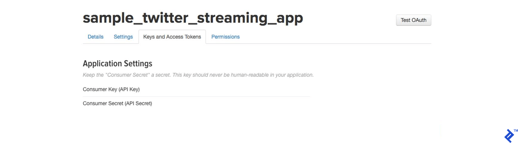
Second, go to your newly created app and open the “Keys and Access Tokens” tab. Then click on “Generate my access token.”
Your new access tokens will appear as below.
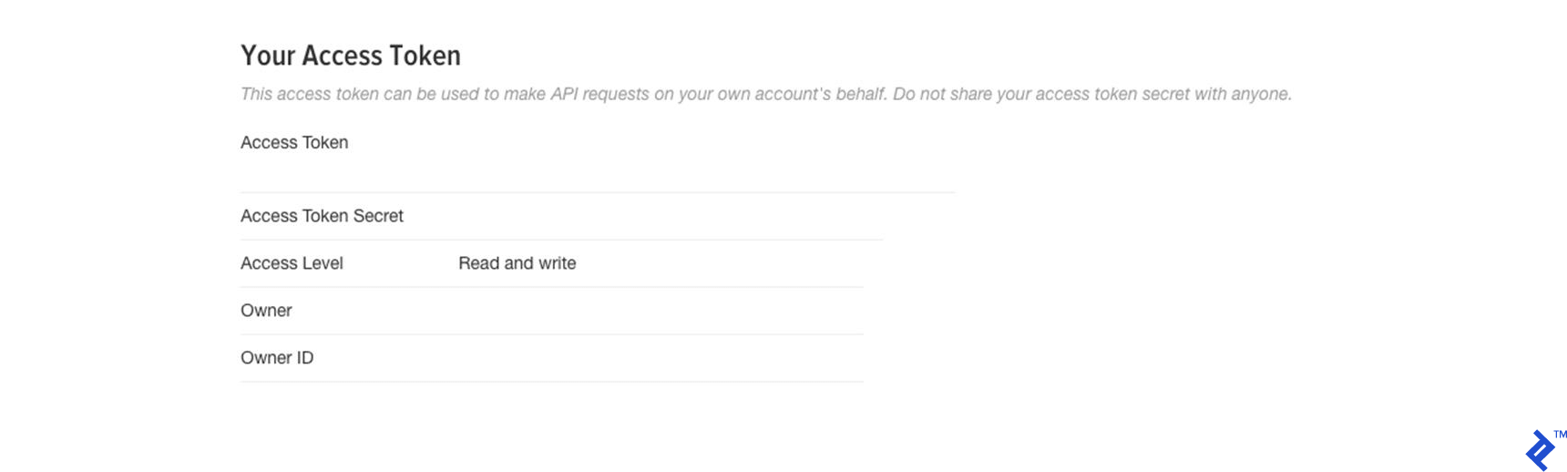
And now you’re ready for the next step.
Building the Twitter HTTP Client
In this step, I’ll show you how to build a simple client that will get the tweets from Twitter API using Python and passes them to the Spark Streaming instance. It should be easy to follow for any professional Python developer.
First, let’s create a file called twitter_app.py and then we’ll add the code in it together as below.
Import the libraries that we’ll use as below:
import socket
import sys
import requests
import requests_oauthlib
import json
And add the variables that will be used in OAuth for connecting to Twitter as below:
# Replace the values below with yours
ACCESS_TOKEN = 'YOUR_ACCESS_TOKEN'
ACCESS_SECRET = 'YOUR_ACCESS_SECRET'
CONSUMER_KEY = 'YOUR_CONSUMER_KEY'
CONSUMER_SECRET = 'YOUR_CONSUMER_SECRET'
my_auth = requests_oauthlib.OAuth1(CONSUMER_KEY, CONSUMER_SECRET,ACCESS_TOKEN, ACCESS_SECRET)
Now, we will create a new function called get_tweets that will call the Twitter API URL and return the response for a stream of tweets.
def get_tweets():
	url = 'https://stream.twitter.com/1.1/statuses/filter.json'
	query_data = [('language', 'en'), ('locations', '-130,-20,100,50'),('track','#')]
	query_url = url + '?' + '&'.join([str(t[0]) + '=' + str(t[1]) for t in query_data])
	response = requests.get(query_url, auth=my_auth, stream=True)
	print(query_url, response)
	return response
Then, create a function that takes the response from the above one and extracts the tweets’ text from the whole tweets’ JSON object. After that, it sends every tweet to Spark Streaming instance (will be discussed later) through a TCP connection.
def send_tweets_to_spark(http_resp, tcp_connection):
	for line in http_resp.iter_lines():
    	try:
        	full_tweet = json.loads(line)
        	tweet_text = full_tweet['text']
        	print("Tweet Text: " + tweet_text)
        	print ("------------------------------------------")
        	tcp_connection.send(tweet_text + '\n')
    	except:
        	e = sys.exc_info()[0]
        	print("Error: %s" % e)
Now, we’ll make the main part which will make the app host socket connections that spark will connect with. We’ll configure the IP here to be localhost as all will run on the same machine and the port 9009. Then we’ll call the get_tweets method, which we made above, for getting the tweets from Twitter and pass its response along with the socket connection to send_tweets_to_spark for sending the tweets to Spark.
TCP_IP = "localhost"
TCP_PORT = 9009
conn = None
s = socket.socket(socket.AF_INET, socket.SOCK_STREAM)
s.bind((TCP_IP, TCP_PORT))
s.listen(1)
print("Waiting for TCP connection...")
conn, addr = s.accept()
print("Connected... Starting getting tweets.")
resp = get_tweets()
send_tweets_to_spark(resp, conn)
Setting Up Our Apache Spark Streaming Application
Let’s build up our Spark streaming app that will do real-time processing for the incoming tweets, extract the hashtags from them, and calculate how many hashtags have been mentioned.

First, we have to create an instance of Spark Context sc, then we created the Streaming Context ssc from sc with a batch interval two seconds that will do the transformation on all streams received every two seconds. Notice we have set the log level to ERROR in order to disable most of the logs that Spark writes.
We defined a checkpoint here in order to allow periodic RDD checkpointing; this is mandatory to be used in our app, as we’ll use stateful transformations (will be discussed later in the same section).
Then we define our main DStream dataStream that will connect to the socket server we created before on port 9009 and read the tweets from that port. Each record in the DStream will be a tweet.
from pyspark import SparkConf,SparkContext
from pyspark.streaming import StreamingContext
from pyspark.sql import Row,SQLContext
import sys
import requests
# create spark configuration
conf = SparkConf()
conf.setAppName("TwitterStreamApp")
# create spark context with the above configuration
sc = SparkContext(conf=conf)
sc.setLogLevel("ERROR")
# create the Streaming Context from the above spark context with interval size 2 seconds
ssc = StreamingContext(sc, 2)
# setting a checkpoint to allow RDD recovery
ssc.checkpoint("checkpoint_TwitterApp")
# read data from port 9009
dataStream = ssc.socketTextStream("localhost",9009)
Now, we’ll define our transformation logic. First we’ll split all the tweets into words and put them in words RDD. Then we’ll filter only hashtags from all words and map them to pair of (hashtag, 1) and put them in hashtags RDD.
Then we need to calculate how many times the hashtag has been mentioned. We can do that by using the function reduceByKey. This function will calculate how many times the hashtag has been mentioned per each batch, i.e. it will reset the counts in each batch.
In our case, we need to calculate the counts across all the batches, so we’ll use another function called updateStateByKey, as this function allows you to maintain the state of RDD while updating it with new data. This way is called Stateful Transformation.
Note that in order to use updateStateByKey, you’ve got to configure a checkpoint, and that what we have done in the previous step.
# split each tweet into words
words = dataStream.flatMap(lambda line: line.split(" "))
# filter the words to get only hashtags, then map each hashtag to be a pair of (hashtag,1)
hashtags = words.filter(lambda w: '#' in w).map(lambda x: (x, 1))
# adding the count of each hashtag to its last count
tags_totals = hashtags.updateStateByKey(aggregate_tags_count)
# do processing for each RDD generated in each interval
tags_totals.foreachRDD(process_rdd)
# start the streaming computation
ssc.start()
# wait for the streaming to finish
ssc.awaitTermination()
The updateStateByKey takes a function as a parameter called the update function. It runs on each item in RDD and does the desired logic.
In our case, we’ve created an update function called aggregate_tags_count that will sum all the new_values for each hashtag and add them to the total_sum that is the sum across all the batches and save the data into tags_totals RDD.
def aggregate_tags_count(new_values, total_sum):
	return sum(new_values) + (total_sum or 0)
Then we do processing on tags_totals RDD in every batch in order to convert it to temp table using Spark SQL Context and then perform a select statement in order to retrieve the top ten hashtags with their counts and put them into hashtag_counts_df data frame.
def get_sql_context_instance(spark_context):
	if ('sqlContextSingletonInstance' not in globals()):
        globals()['sqlContextSingletonInstance'] = SQLContext(spark_context)
	return globals()['sqlContextSingletonInstance']
def process_rdd(time, rdd):
	print("----------- %s -----------" % str(time))
	try:
    	# Get spark sql singleton context from the current context
    	sql_context = get_sql_context_instance(rdd.context)
    	# convert the RDD to Row RDD
    	row_rdd = rdd.map(lambda w: Row(hashtag=w[0], hashtag_count=w[1]))
    	# create a DF from the Row RDD
    	hashtags_df = sql_context.createDataFrame(row_rdd)
    	# Register the dataframe as table
    	hashtags_df.registerTempTable("hashtags")
    	# get the top 10 hashtags from the table using SQL and print them
    	hashtag_counts_df = sql_context.sql("select hashtag, hashtag_count from hashtags order by hashtag_count desc limit 10")
    	hashtag_counts_df.show()
    	# call this method to prepare top 10 hashtags DF and send them
    	send_df_to_dashboard(hashtag_counts_df)
	except:
    	e = sys.exc_info()[0]
    	print("Error: %s" % e)
The last step in our Spark application is to send the hashtag_counts_df data frame to the dashboard application. So we’ll convert the data frame into two arrays, one for the hashtags and the other for their counts. Then we’ll send them to the dashboard application through the REST API.
def send_df_to_dashboard(df):
	# extract the hashtags from dataframe and convert them into array
	top_tags = [str(t.hashtag) for t in df.select("hashtag").collect()]
	# extract the counts from dataframe and convert them into array
	tags_count = [p.hashtag_count for p in df.select("hashtag_count").collect()]
	# initialize and send the data through REST API
	url = 'http://localhost:5001/updateData'
	request_data = {'label': str(top_tags), 'data': str(tags_count)}
	response = requests.post(url, data=request_data)
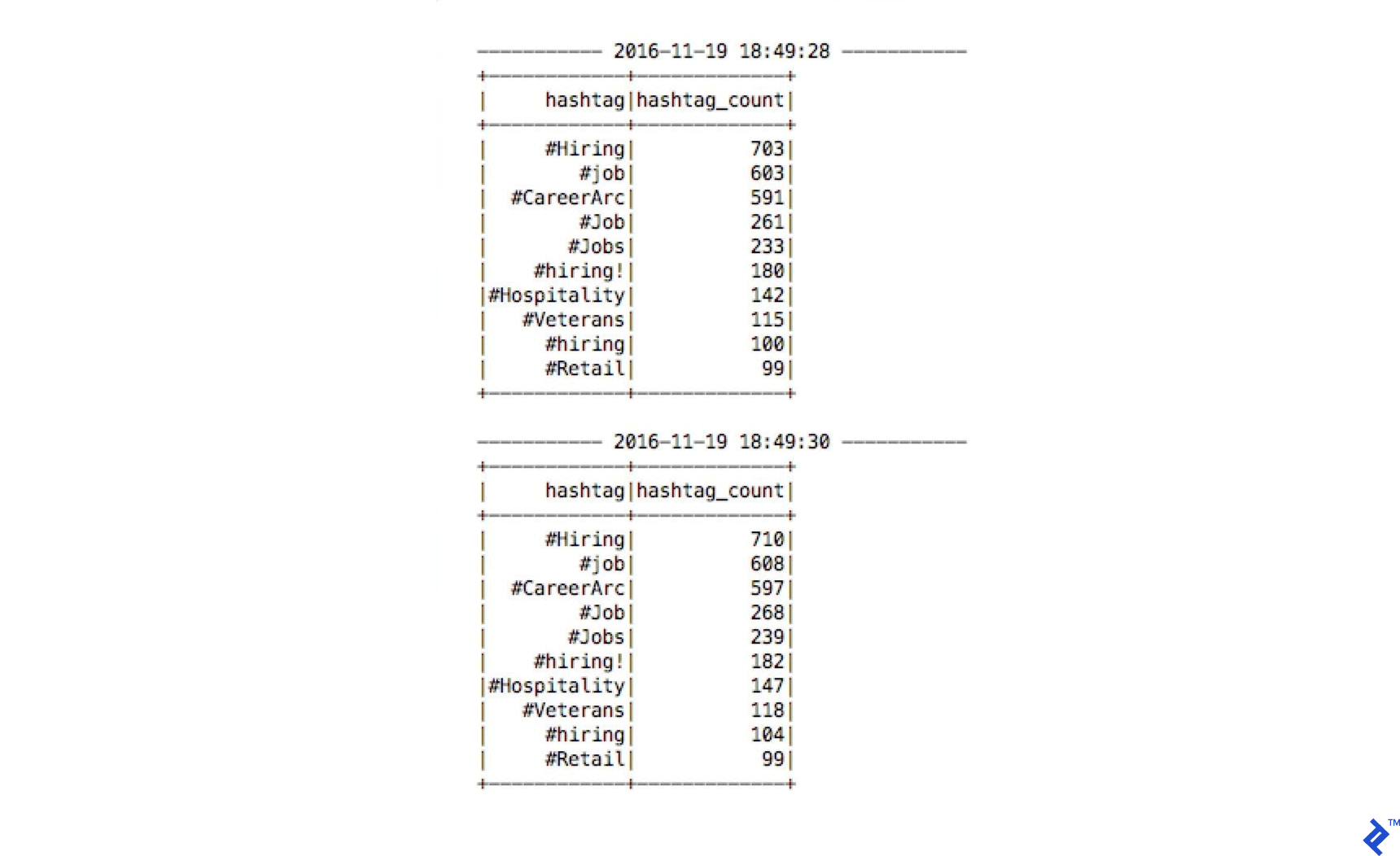
Finally, here is a sample output of the Spark Streaming while running and printing the hashtag_counts_df, you’ll notice that the output is printed exactly every two seconds as per the batch intervals.
Create a Simple Real-time Dashboard for Representing the Data
Now, we’ll create a simple dashboard application that will be updated in real time by Spark. We’ll build it using Python, Flask, and Charts.js.
First, let’s create a Python project with the structure seen below and download and add the Chart.js file into the static directory.
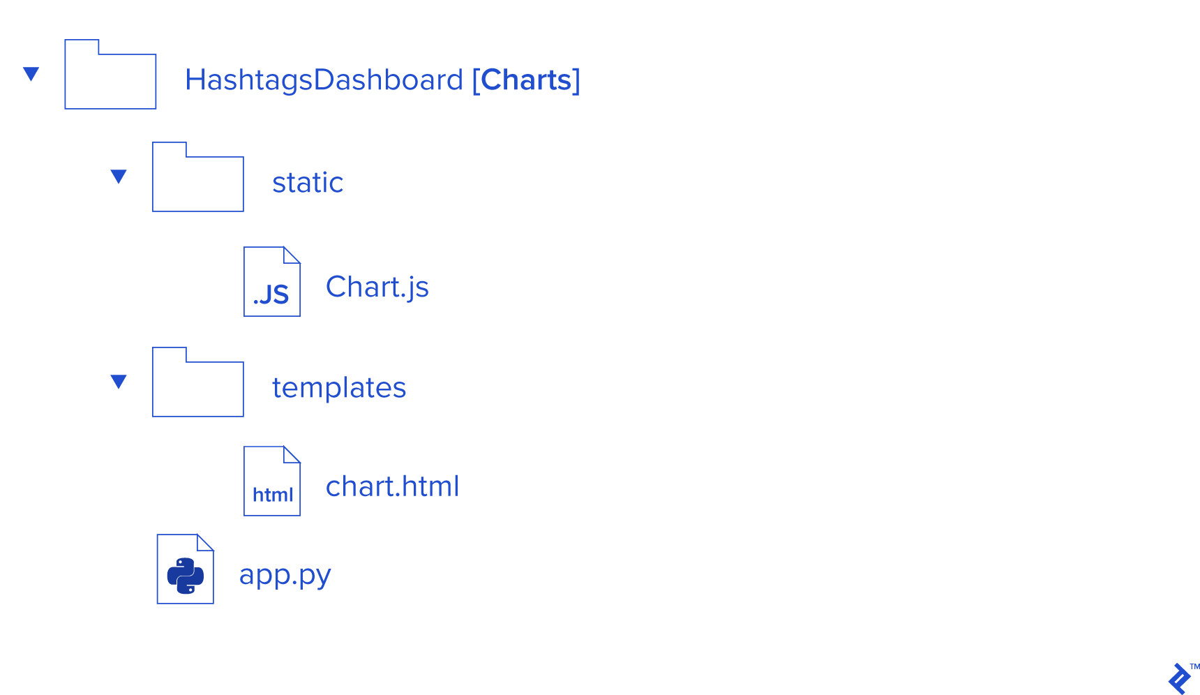
Then, in the app.py file, we’ll create a function called update_data, which will be called by Spark through the URL http://localhost:5001/updateData in order to update the Global labels and values arrays.
Also, the function refresh_graph_data is created to be called by AJAX request to return the new updated labels and values arrays as JSON. The function get_chart_page will render the chart.html page when called.
from flask import Flask,jsonify,request
from flask import render_template
import ast
app = Flask(__name__)
labels = []
values = []
@app.route("/")
def get_chart_page():
	global labels,values
	labels = []
	values = []
	return render_template('chart.html', values=values, labels=labels)
@app.route('/refreshData')
def refresh_graph_data():
	global labels, values
	print("labels now: " + str(labels))
	print("data now: " + str(values))
	return jsonify(sLabel=labels, sData=values)
@app.route('/updateData', methods=['POST'])
def update_data():
	global labels, values
	if not request.form or 'data' not in request.form:
    	return "error",400
	labels = ast.literal_eval(request.form['label'])
	values = ast.literal_eval(request.form['data'])
	print("labels received: " + str(labels))
	print("data received: " + str(values))
	return "success",201
if __name__ == "__main__":
	app.run(host='localhost', port=5001)
Now, let’s create a simple chart in the chart.html file in order to display the hashtag data and update them in real time. As defined below, we need to import the Chart.js and jquery.min.js JavaScript libraries.
In the body tag, we have to create a canvas and give it an ID in order to reference it while displaying the chart using JavaScript in the next step.
<!DOCTYPE html>
<html>
	<head>
    	<meta charset="utf-8"/>
    	<title>Top Trending Twitter Hashtags</title>
    	<script src='static/Chart.js'></script>
    	<script src="//ajax.googleapis.com/ajax/libs/jquery/1.9.1/jquery.min.js"></script>

	</head>
	<body>
        	<h2>Top Trending Twitter Hashtags</h2>
        	<div style="width:700px;height=500px">
            	<canvas id="chart"></canvas>
        	</div>
	</body>
</html>
Now, let’s construct the chart using the JavaScript code below. First, we get the canvas element, and then we create a new chart object and pass the canvas element to it and define its data object like below.
Note that the data’s labels and data are bounded with labels and values variables that are returned while rendering the page when calling a get_chart_page function in the app.py file.
The last remaining part is the function that is configured to do an Ajax request every second and call the URL /refreshData, which will execute refresh_graph_data in app.py and return the new updated data, and then update the char that renders the new data.
<script>
   var ctx = document.getElementById("chart");
   var myChart = new Chart(ctx, {
    	type: 'horizontalBar',
    	data: {
        	labels: [{% for item in labels %}
                  	"{{item}}",
                 	{% endfor %}],
        	datasets: [{
            	label: '# of Mentions',
            	data: [{% for item in values %}
     	                 {{item}},
                    	{% endfor %}],
            	backgroundColor: [
                	'rgba(255, 99, 132, 0.2)',
                	'rgba(54, 162, 235, 0.2)',
                	'rgba(255, 206, 86, 0.2)',
          	      'rgba(75, 192, 192, 0.2)',
                	'rgba(153, 102, 255, 0.2)',
                	'rgba(255, 159, 64, 0.2)',
                	'rgba(255, 99, 132, 0.2)',
                	'rgba(54, 162, 235, 0.2)',
                	'rgba(255, 206, 86, 0.2)',
                	'rgba(75, 192, 192, 0.2)',
                	'rgba(153, 102, 255, 0.2)'
            	],
            	borderColor: [
                	'rgba(255,99,132,1)',
                	'rgba(54, 162, 235, 1)',
        	        'rgba(255, 206, 86, 1)',
                	'rgba(75, 192, 192, 1)',
                	'rgba(153, 102, 255, 1)',
                	'rgba(255, 159, 64, 1)',
                	'rgba(255,99,132,1)',
                	'rgba(54, 162, 235, 1)',
                	'rgba(255, 206, 86, 1)',
                	'rgba(75, 192, 192, 1)',
                	'rgba(153, 102, 255, 1)'
            	],
            	borderWidth: 1
        	}]
    	},
    	options: {
        	scales: {
	            yAxes: [{
                	ticks: {
                    	beginAtZero:true
                	}
            	}]
        	}
    	}
   });
   var src_Labels = [];
   var src_Data = [];
   setInterval(function(){
    	$.getJSON('/refreshData', {
    	}, function(data) {
        	src_Labels = data.sLabel;
        	src_Data = data.sData;
    	});
    	myChart.data.labels = src_Labels;
    	myChart.data.datasets[0].data = src_Data;
    	myChart.update();
   },1000);
</script>
Running the applications together
Let’s run the three applications in the order below: 1. Twitter App Client. 2. Spark App. 3. Dashboard Web App.
Then you can access the real-time dashboard using the URL <http://localhost:5001/>
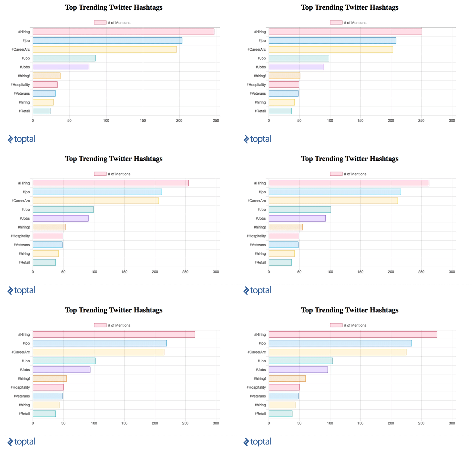
Now, you can see your chart being updated, as below: